B-estimate writes when the script runsDictionary of Applied Machine Learning · mean squared error (MSE)
Updated on 2026-11-20
Numerical companion to the entry mean squared error (MSE): it recomputes what the entry states and prints one line per check
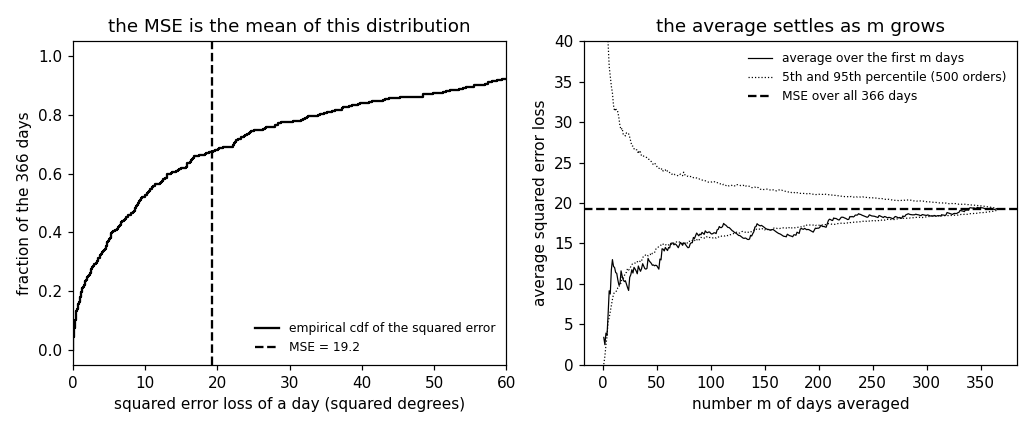
Numerical companion to the glossary entry 'mse' (mean squared error). A linear hypothesis that predicts the maximum daytime temperature from the morning minimum is learned by least squares on the 365 days of 2023 at Krems (GeoSphere station 3805). Its MSE is then computed on the 366 days of 2024 in the two forms the entry writes down: as the average of the squared error loss over the days, and as the expectation of the squared error loss when a day is drawn from the empirical distribution of the 2024 days, which puts probability 1/m on each day. The two agree exactly; that is the point of the entry. The demo also shows the average over the first m days settling towards the 366-day value, the sense in which the dataset average estimates the MSE as an expectation under the data-generating distribution.
Run it without installing anything:uv run https://dictionaryofml.org/terms/mse.py
uv downloads this script and the pinned NumPy and Matplotlib it needs, then runs it; the script fetches any input file it uses. To keep the output files, download mse.py into a folder and run uv run mse.py there. With NumPy and Matplotlib already installed, python3 mse.py, from any directory — it writes its output files into the current directory. Fixed seeds, so the printed numbers reproduce exactly. Download mse.py · Notebook · Open in Colab
Before running a downloaded copy, scan it: uvx bandit -q -t B102,B307,B602,B605 mse.py (B102,B307,B602,B605 are the exec, eval and shell checks of bandit) reports nothing: the script runs no shell command and evaluates no generated code.
One cell per block of the script: the code, and what that code printed when it last ran here
"""The mean squared error (MSE) of a temperature hypothesis at Krems an der
Donau: the average squared error loss over a dataset, and the same number
as an expectation under the empirical distribution of that dataset.

Purpose
-------
Numerical companion to the glossary entry 'mse' (mean squared error).  A
linear hypothesis that predicts the maximum daytime temperature from the
morning minimum is learned by least squares on the 365 days of 2023 at
Krems (GeoSphere station 3805).  Its MSE is then computed on the 366 days
of 2024 in the two forms the entry writes down: as the average of the
squared error loss over the days, and as the expectation of the squared
error loss when a day is drawn from the empirical distribution of the
2024 days, which puts probability 1/m on each day.  The two agree
exactly; that is the point of the entry.  The demo also shows the
average over the first m days settling towards the 366-day value, the
sense in which the dataset average estimates the MSE as an expectation
under the data-generating distribution.

Self-contained (numpy and matplotlib only), fixed seeds; the GeoSphere
download falls back to the committed CSV.

Blocks
------
[B-data]     Daily minimum and maximum temperature at Krems for 2023 and
             2024 (731 days, no missing value).
[B-learn]    Least squares on the 2023 days gives the linear hypothesis;
             its MSE on the training days.
[B-average]  The MSE on the 2024 days as the average of the per-day
             squared error loss; the root MSE in degrees.
[B-empdist]  The same number as an expectation: probability 1/366 per day
             (duplicates merged into their multiplicities), the mean of
             the empirical distribution of the squared errors.
[B-estimate] The average over the first m days of 2024 in a random
             order, and the 5th to 95th percentile band of that average
             over 500 orders, against the 366-day MSE.
[B-robust]   What the squaring costs: the MAE of the same hypothesis, the
             constant prediction each of the two averages prefers (the
             mean of the labels against their median), and how far one
             mismeasured day moves each of the two.

Outputs
-------
mse_weather.csv   : date, tmin, tmax for 2023 and 2024 (committed copy).
mse_cdf.csv       : squared error of each 2024 day, sorted, with the
                    empirical cdf value.
mse_running.csv   : m, running average for one order, 5th and 95th
                    percentile of the running average over 500 orders.
mse_robust.csv    : size of a single recording error in degrees, and the
                    shift it causes in the MSE-optimal and the MAE-optimal
                    constant prediction.
mse.png           : matplotlib preview (checking only).
"""

# /// script
# requires-python = ">=3.10"
# dependencies = ["matplotlib==3.10.7", "numpy==2.3.4"]
# ///

import json
import urllib.request
from pathlib import Path

import numpy as np
import matplotlib

matplotlib.use("Agg")
import matplotlib.pyplot as plt

OUT_DIR = Path(__file__).parent

report = []


def check(name, ok):
    report.append((name, bool(ok)))
    print(f"  [{'ok' if ok else 'FAIL'}] {name}")
Daily minimum and maximum temperature at Krems for 2023 and 2024 (731 days, no missing value).
print("[B-data] daily minimum and maximum temperature at Krems, 2023 and 2024")
URL = ("https://dataset.api.hub.geosphere.at/v1/station/historical/"
       "klima-v2-1d?parameters=tlmin,tlmax&station_ids=3805"
       "&start=2023-01-01&end=2024-12-31")
CSV = OUT_DIR / "mse_weather.csv"
try:
    with urllib.request.urlopen(URL, timeout=120) as resp:
        payload = json.load(resp)
    params = payload["features"][0]["properties"]["parameters"]
    records = [(stamp[:10], lo, hi)
               for stamp, lo, hi in zip(payload["timestamps"],
                                        params["tlmin"]["data"],
                                        params["tlmax"]["data"])]
    with open(CSV, "w") as fh:
        fh.write("date,tmin,tmax\n")
        for day, lo, hi in records:
            fh.write(f"{day},{lo},{hi}\n")
    print(f"    downloaded {len(records)} days")
except OSError as err:
    print(f"    download failed ({err}); reading the committed CSV")
    rows = CSV.read_text().strip().splitlines()[1:]
    records = [(d, float(a), float(b))
               for d, a, b in (r.split(",") for r in rows)]

check("[B-data] 731 days for 2023 and 2024", len(records) == 731)
check("[B-data] no day is missing a temperature",
      all(lo is not None and hi is not None for _, lo, hi in records))
x = np.array([lo for _, lo, _ in records])
y = np.array([hi for _, _, hi in records])
is23 = np.array([d.startswith("2023") for d, _, _ in records])
x23, y23, x24, y24 = x[is23], y[is23], x[~is23], y[~is23]
m23, m24 = len(x23), len(x24)
[B-data] daily minimum and maximum temperature at Krems, 2023 and 2024
    downloaded 731 days
  [ok] [B-data] 731 days for 2023 and 2024
  [ok] [B-data] no day is missing a temperature
Least squares on the 2023 days gives the linear hypothesis; its MSE on the training days.
print("[B-learn] linear hypothesis learned on the 2023 days")
A = np.column_stack([np.ones(m23), x23])
w0, w1 = np.linalg.lstsq(A, y23, rcond=None)[0]


def h(xx):
    return w0 + w1 * xx


mse23 = float(np.mean((y23 - h(x23)) ** 2))
check(f"[B-learn] h(x) = {w0:.2f} + {w1:.3f} x; MSE on the 365 training "
      f"days {mse23:.2f}", 0.5 < w1 < 1.5 and mse23 > 0)
[B-learn] linear hypothesis learned on the 2023 days
  [ok] [B-learn] h(x) = 9.81 + 1.137 x; MSE on the 365 training days 21.06
The MSE on the 2024 days as the average of the per-day squared error loss; the root MSE in degrees.
print("[B-average] MSE on the 2024 days as the average squared error loss")
sq = (y24 - h(x24)) ** 2                       # per-day squared error loss
mse24 = float(np.mean(sq))
check(f"[B-average] MSE on the 366 days of 2024: {mse24:.2f} squared "
      f"degrees, root MSE {np.sqrt(mse24):.2f} degrees", mse24 > 0)
check(f"[B-average] the loss of 1 January 2024 (minimum {x24[0]:.1f}, "
      f"maximum {y24[0]:.1f}, prediction {h(x24[0]):.2f}) is "
      f"{sq[0]:.2f}", abs(sq[0] - (y24[0] - h(x24[0])) ** 2) < 1e-12)
check(f"[B-average] the MSE of 2024 is {'above' if mse24 > mse23 else 'below'}"
      f" the training MSE of 2023 ({mse24:.2f} against {mse23:.2f})", True)
[B-average] MSE on the 2024 days as the average squared error loss
  [ok] [B-average] MSE on the 366 days of 2024: 19.25 squared degrees, root MSE 4.39 degrees
  [ok] [B-average] the loss of 1 January 2024 (minimum 2.6, maximum 9.6, prediction 12.76) is 10.00
  [ok] [B-average] the MSE of 2024 is below the training MSE of 2023 (19.25 against 21.06)
The same number as an expectation: probability 1/366 per day (duplicates merged into their multiplicities), the mean of the empirical distribution of the squared errors.
#      empirical distribution of the 2024 days
print("[B-empdist] expectation under the empirical distribution")
pairs = {}
for xi, yi in zip(x24, y24):
    pairs[(xi, yi)] = pairs.get((xi, yi), 0) + 1
check(f"[B-empdist] {len(pairs)} distinct (minimum, maximum) pairs among "
      f"the 366 days; the empirical distribution gives each pair the "
      f"probability (multiplicity)/366", sum(pairs.values()) == m24)
expectation = sum(n / m24 * (yi - h(xi)) ** 2 for (xi, yi), n in pairs.items())
check(f"[B-empdist] expectation {expectation:.6f} equals the average "
      f"{mse24:.6f}", abs(expectation - mse24) < 1e-9)
order = np.argsort(sq)
sq_sorted, cdf = sq[order], np.arange(1, m24 + 1) / m24
median = float(sq_sorted[m24 // 2 - 1 + m24 % 2])
check(f"[B-empdist] the empirical distribution of the squared errors is "
      f"skewed: median {median:.2f}, mean {mse24:.2f}, largest "
      f"{sq_sorted[-1]:.1f}; {100 * np.mean(sq < mse24):.0f}% of the days "
      f"have a loss below the MSE", median < mse24 < sq_sorted[-1])
[B-empdist] expectation under the empirical distribution
  [ok] [B-empdist] 364 distinct (minimum, maximum) pairs among the 366 days; the empirical distribution gives each pair the probability (multiplicity)/366
  [ok] [B-empdist] expectation 19.246414 equals the average 19.246414
  [ok] [B-empdist] the empirical distribution of the squared errors is skewed: median 9.06, mean 19.25, largest 117.2; 67% of the days have a loss below the MSE
The average over the first m days of 2024 in a random order, and the 5th to 95th percentile band of that average over 500 orders, against the 366-day MSE.
print("[B-estimate] running average against the 366-day MSE")
rng = np.random.default_rng(2024)
R = 500
run = np.empty((R, m24))
for r in range(R):
    perm = rng.permutation(m24)
    run[r] = np.cumsum(sq[perm]) / np.arange(1, m24 + 1)
lo, hi = np.percentile(run, 5, axis=0), np.percentile(run, 95, axis=0)
one = run[0]
check(f"[B-estimate] every running average ends at the MSE {mse24:.2f}",
      np.allclose(run[:, -1], mse24))
check(f"[B-estimate] 5th to 95th percentile of the average over the first "
      f"30 days: [{lo[29]:.1f}, {hi[29]:.1f}]; over the first 180 days: "
      f"[{lo[179]:.1f}, {hi[179]:.1f}]",
      hi[29] - lo[29] > hi[179] - lo[179] > 0)
check("[B-estimate] the band narrows with m (monotone from m = 10 on,"
      " up to small reversals below 1 squared degree)",
      np.all(np.diff((hi - lo)[9:]) < 1.0))

# ---- CSVs and preview
with open(OUT_DIR / "mse_cdf.csv", "w") as fh:
    fh.write("sqerr,cdf\n")
    for s, c in zip(sq_sorted, cdf):
        fh.write(f"{s:.4f},{c:.6f}\n")
with open(OUT_DIR / "mse_running.csv", "w") as fh:
    fh.write("m,running,lo,hi\n")
    for i in range(m24):
        fh.write(f"{i + 1},{one[i]:.4f},{lo[i]:.4f},{hi[i]:.4f}\n")

fig, (ax1, ax2) = plt.subplots(1, 2, figsize=(9.4, 3.9))
ax1.step(np.concatenate([[0], sq_sorted]), np.concatenate([[0], cdf]),
         where="post", color="black", label="empirical cdf of the squared error")
ax1.axvline(mse24, color="black", ls="--", label=f"MSE = {mse24:.1f}")
ax1.set_xlim(0, 60)
ax1.set_xlabel("squared error loss of a day (squared degrees)")
ax1.set_ylabel("fraction of the 366 days")
ax1.set_title("the MSE is the mean of this distribution")
ax1.legend(frameon=False, fontsize=8)
ax2.plot(np.arange(1, m24 + 1), one, "k-", lw=0.8, label="average over the first m days")
ax2.plot(np.arange(1, m24 + 1), lo, "k:", lw=0.8, label="5th and 95th percentile (500 orders)")
ax2.plot(np.arange(1, m24 + 1), hi, "k:", lw=0.8)
ax2.axhline(mse24, color="black", ls="--", label="MSE over all 366 days")
ax2.set_ylim(0, 40)
ax2.set_xlabel("number m of days averaged")
ax2.set_ylabel("average squared error loss")
ax2.set_title("the average settles as m grows")
ax2.legend(frameon=False, fontsize=8)
fig.tight_layout()
fig.savefig(OUT_DIR / "mse.png", dpi=110)
[B-estimate] running average against the 366-day MSE
  [ok] [B-estimate] every running average ends at the MSE 19.25
  [ok] [B-estimate] 5th to 95th percentile of the average over the first 30 days: [12.6, 26.7]; over the first 180 days: [17.0, 21.3]
  [ok] [B-estimate] the band narrows with m (monotone from m = 10 on, up to small reversals below 1 squared degree)
B-estimate writes when the script runsWhat the squaring costs: the MAE of the same hypothesis, the constant prediction each of the two averages prefers (the mean of the labels against their median), and how far one mismeasured day moves each of the two.
print("[B-robust] the squared average against the absolute average")
mae24 = float(np.mean(np.abs(y24 - h(x24))))
check(f"[B-robust] MAE of the same hypothesis on the 366 days of 2024: "
      f"{mae24:.2f} degrees, against a root MSE of {np.sqrt(mse24):.2f}",
      mae24 < np.sqrt(mse24))

# a constant prediction: the squared average prefers the mean of the
# labels, the absolute average their median
grid = np.linspace(y24.min(), y24.max(), 20001)
c_sq = float(grid[np.argmin([np.mean((y24 - c) ** 2) for c in grid[::50]][0:0] or
                            np.mean((y24[:, None] - grid[None, :]) ** 2, axis=0))])
c_ab = float(grid[np.argmin(np.mean(np.abs(y24[:, None] - grid[None, :]),
                                    axis=0))])
check(f"[B-robust] over a grid of {grid.size} constants, the squared "
      f"average is smallest at {c_sq:.2f} and the mean of the labels is "
      f"{y24.mean():.2f}", abs(c_sq - y24.mean()) < 0.02)
check(f"[B-robust] the absolute average is smallest at {c_ab:.2f} and "
      f"the median of the labels is {np.median(y24):.2f}",
      abs(c_ab - np.median(y24)) < 0.02)

# one mismeasured day, by a decimal point or a sensor fault
shifts, rows = [5.0, 10.0, 20.0, 50.0], []
for s_deg in shifts:
    y_bad = y24.copy()
    y_bad[0] += s_deg
    d_sq = abs(float(y_bad.mean()) - float(y24.mean()))
    d_ab = abs(float(np.median(y_bad)) - float(np.median(y24)))
    rows.append((s_deg, d_sq, d_ab))
    check(f"[B-robust] moving one of the {m24} labels by {s_deg:.0f} "
          f"degrees moves the mean by {d_sq:.3f} and the median by "
          f"{d_ab:.3f} degrees",
          abs(d_sq - s_deg / m24) < 1e-9)
# the mean moves by the error divided by the sample size, without bound;
# the median moves at most to the neighboring label and then stops, so a
# gross error has a bounded effect on it
gap = float(np.diff(np.sort(y24))[np.searchsorted(
    np.sort(y24), np.median(y24)) - 1:][0:1].max())
check(f"[B-robust] the shift of the mean grows in proportion to the "
      f"error ({rows[0][1]:.3f} to {rows[-1][1]:.3f} degrees, each the "
      f"error divided by {m24}) while the shift of the median stops at "
      f"{max(r[2] for r in rows):.3f}, the step to the neighboring "
      f"label", rows[-1][1] > 9 * rows[0][1]
      and max(r[2] for r in rows) <= gap + 1e-9)
check(f"[B-robust] from a {shifts[1]:.0f} degree error on, the median "
      f"no longer moves further: {rows[1][2]:.3f}, {rows[2][2]:.3f}, "
      f"{rows[3][2]:.3f} degrees",
      abs(rows[1][2] - rows[3][2]) < 1e-9)
np.savetxt(OUT_DIR / "mse_robust.csv",
           np.array(rows), delimiter=",", fmt="%.6f",
           header="shift,mean_shift,median_shift", comments="")

n_ok = sum(ok for _, ok in report)
print(f"\n{n_ok}/{len(report)} checks pass")
if n_ok != len(report):
    raise SystemExit(1)
[B-robust] the squared average against the absolute average
  [ok] [B-robust] MAE of the same hypothesis on the 366 days of 2024: 3.55 degrees, against a root MSE of 4.39
  [ok] [B-robust] over a grid of 20001 constants, the squared average is smallest at 17.91 and the mean of the labels is 17.91
  [ok] [B-robust] the absolute average is smallest at 17.60 and the median of the labels is 17.60
  [ok] [B-robust] moving one of the 366 labels by 5 degrees moves the mean by 0.014 and the median by 0.000 degrees
  [ok] [B-robust] moving one of the 366 labels by 10 degrees moves the mean by 0.027 and the median by 0.100 degrees
  [ok] [B-robust] moving one of the 366 labels by 20 degrees moves the mean by 0.055 and the median by 0.100 degrees
  [ok] [B-robust] moving one of the 366 labels by 50 degrees moves the mean by 0.137 and the median by 0.100 degrees
  [ok] [B-robust] the shift of the mean grows in proportion to the error (0.014 to 0.137 degrees, each the error divided by 366) while the shift of the median stops at 0.100, the step to the neighboring label
  [ok] [B-robust] from a 10 degree error on, the median no longer moves further: 0.100, 0.100, 0.100 degrees

21/21 checks pass