randomprojection.py, which recomputes what the entry states: the script block by block · open in ColabDictionary of Applied Machine Learning: 147 machine-learning terms, each with a definition, a figure, citations and a Python demo · All terms · Demos · Start here
Updated on 2026-11-19
Readiness 85/100
See also dimensionality reduction feature learning principal component analysis autoencoder feature vector
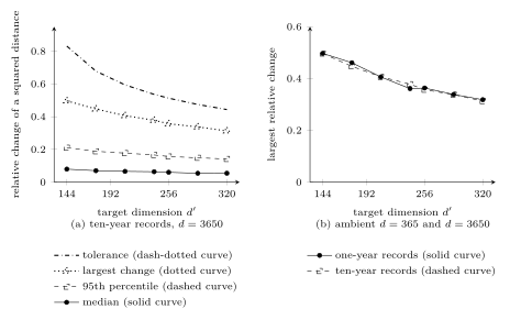
A random projection replaces the feature vector ${\mathbf x} \in \mathbb{R}^{d}$ of a data point by ${\mathbf A} {\mathbf x} \in \mathbb{R}^{d'}$, with $d' < d$ and a wide matrix ${\mathbf A}$ whose entries are realizations of independent and identically distributed (i.i.d.) random variables (RVs). No data enter ${\mathbf A}$, which separates a random projection from principal component analysis (PCA) and from an autoencoder, whose maps for dimensionality reduction are learned from a training set. When the entries have mean zero and variance $1/d'$, the expectation of the squared length of ${\mathbf A} {\mathbf x}$ equals the squared length of ${\mathbf x}$, so squared Euclidean distances between data points survive on average. The Johnson–Lindenstrauss lemma (JL lemma) turns this into a guarantee for a whole finite dataset: a target dimension of at least $4 \ln m / (\varepsilon^{2}/2 - \varepsilon^{3}/3)$ keeps every pairwise squared Euclidean distance within the factor $1 \pm \varepsilon$. That requirement involves the sample size $m$ and the tolerance $\varepsilon$ and not the ambient dimension $d$, so the saving grows with the length of the original feature vector. The entries may be normal RVs or take the values $\pm 1/\sqrt{d'}$ with probability one half each. A random projection costs one matrix multiplication per data point and no pass over the data.
randomprojection.py, which recomputes what the entry states: the script block by block · open in ColabB-dataA weather archive at Krems an der Donau (Austria) keeps, for each day, the daily maximum air temperature of the preceding ten years. Such a day is a data point whose feature vector ${\mathbf x} \in \mathbb{R}^{d}$ holds $d = 3650$ numbers, and a search for the days most similar to a given one compares these feature vectors by their Euclidean distance. A random projection shortens every record before the search: it replaces ${\mathbf x}$ by ${\mathbf A} {\mathbf x} \in \mathbb{R}^{d'}$, where $d' < d$ and ${\mathbf A} \in \mathbb{R}^{d' \times d}$ is a wide matrix whose entries are realizations of independent and identically distributed (i.i.d.) random variables (RVs). No data enter ${\mathbf A}$, and that is what separates a random projection from principal component analysis (PCA) and from an autoencoder, whose maps for dimensionality reduction are learned from a training set. The word projection is traditional here: the matrix ${\mathbf A}$ maps into $\mathbb{R}^{d'}$, so it is not a projection of $\mathbb{R}^{d}$ onto one of its subsets.
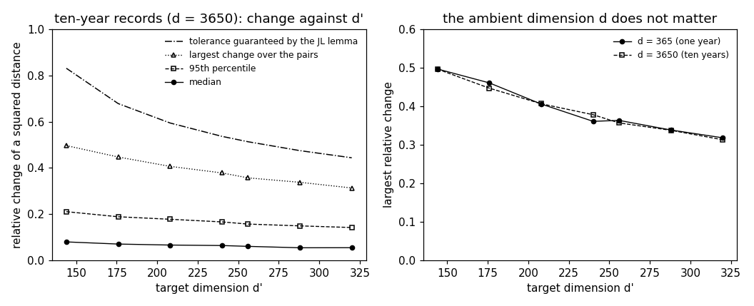
B-expectThe probability distribution of these RVs has mean zero and variance $1/d'$. Consider a fixed ${\mathbf u} \in \mathbb{R}^{d}$. Each entry of ${\mathbf A} {\mathbf u}$ is then an RV with mean zero and variance $\left\lVert {\mathbf u} \right\rVert_{2}^{2}/d'$. Adding the variances of the $d'$ entries gives the expectation of the squared length of ${\mathbf A} {\mathbf u}$, \begin{equation} \label{equ_randomprojection_isometry_dict} \mathbb{E} \big\{ \left\lVert {\mathbf A} {\mathbf u} \right\rVert_{2}^{2} \big\} = \left\lVert {\mathbf u} \right\rVert_{2}^{2} \text{.} \end{equation} Read with ${\mathbf u} = {\mathbf x}^{(r)} - {\mathbf x}^{(r')}$, the identity \(\eqref{equ_randomprojection_isometry_dict}\) says that the squared Euclidean distance between two data points survives the projection on average. One draw of ${\mathbf A}$ is another matter. For two of the Krems days and $d' = 16$, the squared Euclidean distance after the projection ranged from $0.22$ to $2.68$ times the one before it over $4000$ draws.
B-distortThat spread narrows as $d'$ grows, and the
Johnson–Lindenstrauss lemma (JL lemma), proved by
Johnson and Lindenstrauss (1984), turns the narrowing into a
guarantee that covers every pair of a finite dataset at
once.
Consider a dataset $\mathcal{D} = \{{\mathbf x}^{(1)}, \ldots,
{\mathbf x}^{(m)}\}$ of sample size $m$
and a tolerance $\varepsilon$ with $0 < \varepsilon < 1$. Whenever
the target dimension satisfies
\begin{equation}
\label{equ_randomprojection_jldim_dict}
d' \ge \frac{4 \ln m}
{\varepsilon^{2}/2 - \varepsilon^{3}/3} \text{,}
\end{equation}
there is a map ${\mathbf \Phi} \colon \mathbb{R}^{d} \to
\mathbb{R}^{d'}$ with
\begin{equation}
\label{equ_randomprojection_jldist_dict}
(1 - \varepsilon) \left\lVert {\mathbf x}^{(r)} -
{\mathbf x}^{(r')} \right\rVert_{2}^{2}
\le \left\lVert {\mathbf \Phi} \big(
{\mathbf x}^{(r)} \big) - {\mathbf \Phi} \big(
{\mathbf x}^{(r')} \big) \right\rVert_{2}^{2}
\le (1 + \varepsilon) \left\lVert {\mathbf x}^{(r)} -
{\mathbf x}^{(r')} \right\rVert_{2}^{2} \text{,}
\end{equation}
for every $r, r' \in \{1, \ldots,
m\}$, and a random projection delivers such a map with
positive probability, which repeated draws raise as high as
wanted (Dasgupta and Gupta, 2003, Thm. 2.1). The requirement
\(\eqref{equ_randomprojection_jldim_dict}\) involves the
sample size $m$ and the tolerance $\varepsilon$, and
not the ambient dimension $d$. Its denominator is largest
at $\varepsilon = 1$, where it equals $1/6$, so no tolerance below
one is granted before $d' \ge 24 \ln m$, which
is $134$ for $m = 256$ days. The sample size enters
through its logarithm: at $\varepsilon = 1/2$, a hundredfold larger
dataset raises the requirement from $266$ to $487$.
Fig. 1 holds the two-sided bound
\(\eqref{equ_randomprojection_jldist_dict}\) against what one draw of
${\mathbf A}$ does to the $32640$ pairwise squared Euclidean distances of
$256$ such days.
pythondemos/randomprojection.py
B-storageFor the Krems archive and $d' = 256$, the ten-year record of a day shrinks from $3650$ numbers to $256$, a factor of $14.3$. In a typical draw of ${\mathbf A}$, no pair of the $32640$ squared Euclidean distances changes by more than $36$ percent and half of them change by less than $6$ percent, against the $51$ percent the requirement \(\eqref{equ_randomprojection_jldim_dict}\) grants at that target dimension. A method that reads the data points only through their pairwise Euclidean distances, such as $k$-nearest neighbors ($k$-NN), therefore works on nearly the dataset it would have worked on before. When both the map and the reconstruction are linear, PCA is the choice with the smallest average squared error over the training set, and a random projection is not. When the step back to $\mathbb{R}^{d}$ may be nonlinear, the ranking can turn around: feature vectors with few nonzero features are recovered better from a random projection than from PCA (Shalev-Shwartz and Ben-David, 2014, Sect. 23.5).
See also: dimensionality reduction, feature learning, Johnson–Lindenstrauss lemma, principal component analysis, autoencoder, random matrix, wide matrix, Euclidean distance, feature vector, $k$-nearest neighbors.
@misc{dictml_randomprojection,
  author = {Jung, Alexander},
  editor = {Olioumtsevits, Konstantina and Schnoor, Ekkehard},
  title = {random projection},
  howpublished = {Dictionary of Applied Machine Learning (course edition)},
  year = {2026},
  doi = {10.5281/zenodo.21569296},
  note = {ISBN 978-952-64-3013-3, CC BY 4.0, retrieved 2026-11-20},
  url = {https://dictionaryofml.org/terms/randomprojection.html}
}