projection

Jung, Alexander

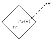
The projection of a vector onto a closed non-empty subset of a Euclidean space is a point in the subset that is closest to the vector in the Euclidean norm. If the subset is convex, this closest point is unique and the solution of a convex optimization problem. If the subset is a subspace, the projection is a linear map, namely the orthogonal projection onto the subspace. Every projection is idempotent, and a linear map of a Hilbert space into itself is an orthogonal projection if and only if the map is idempotent and self-adjoint. In machine learning (ML), projections enforce constraints on model parameters during training: projected gradient descent (projected GD) alternates gradient steps with projections onto the constraint set, e.g., the $\ell_{1}$-ball in an equivalent formulation of the least absolute shrinkage and selection operator (Lasso).

Definition

The least absolute shrinkage and selection operator (Lasso) learns a linear model whose model parameters ${\mathbf w}$ must keep an $\ell_{1}$-norm below a prescribed bound, and a gradient step can move ${\mathbf w}$ outside this set. The result must then be replaced by a closest admissible vector, and training any machine learning (ML) model under a constraint set faces the same replacement at every step. The projection formalizes this replacement.

P-defConsider a non-empty closed set $\mathcal{W} \subseteq \mathbb{R}^{d}$ in the $d$-dimensional Euclidean space. The projection $P_{\mathcal{W}}\big( {\mathbf w}\big)$ of a vector ${\mathbf w} \in \mathbb{R}^{d}$ onto $\mathcal{W}$ is \[ P_{\mathcal{W}}\big( {\mathbf w}\big) = \mathop{\mathrm{arg\,min}}_{{\mathbf w}' \in \mathcal{W}} \left\lVert {\mathbf w} - {\mathbf w}' \right\rVert_{2}\text{,} \] a vector in $\mathcal{W}$ closest to ${\mathbf w}$ in the Euclidean norm. The minimum exists for every non-empty closed set $\mathcal{W}$, but several closest vectors can exist. For the two-point set $\mathcal{W} = \big\{ (-1,0)^{\top}, (1,0)^{\top} \big\}$, both elements are closest to $(0,0.7)^{\top}$, and likewise to every other point on the vertical axis, which consists of exactly the points equidistant from the two elements. If $\mathcal{W}$ is closed and convex, the closest point in the Euclidean norm is unique (Boyd and Vandenberghe, 2004, Sect. 8.1).

The construction extends beyond the Euclidean space: a non-empty closed convex subset of a Hilbert space contains, for each point of the space, a unique closest point (Bauschke and Combettes, 2011, Thm. 3.14). If $\mathcal{W}$ is a subspace, that is, a subset that contains all sums and scalar multiples of its elements (such as a line through the origin), the map ${\mathbf w} \mapsto P_{\mathcal{W}}\big( {\mathbf w}\big)$ is a linear map: it is the orthogonal projection onto $\mathcal{W}$.

P-fundEvery projection is idempotent: the vector $P_{\mathcal{W}}\big( {\mathbf w}\big)$ lies in $\mathcal{W}$, so its closest point in $\mathcal{W}$ is itself and $P_{\mathcal{W}}\big( P_{\mathcal{W}}\big( {\mathbf w}\big)\big) = P_{\mathcal{W}}\big( {\mathbf w}\big)$. A linear map $P$ of a Hilbert space into itself is the orthogonal projection onto the range of $P$ if and only if $P$ is idempotent and self-adjoint, i.e., $\langle P{\mathbf u}, {\mathbf v} \rangle = \langle {\mathbf u}, P{\mathbf v} \rangle$ for all ${\mathbf u}, {\mathbf v}$ (Axler, 2024, Sect. 6C, Exercise 9, and Sect. 7A, Exercise 19). For a matrix $\mathbf{P} \in \mathbb{R}^{d \times d}$ acting on the Euclidean space, idempotence is the condition $\mathbf{P}^{2} = \mathbf{P}$ and self-adjointness the condition $\mathbf{P}^{\top} = \mathbf{P}$. Idempotence alone is not sufficient for a linear map to be an orthogonal projection: an idempotent linear map that is not self-adjoint is an oblique projection (Meyer, 2000, Sect. 5.9). For example, the matrix $\mathbf{P} = \begin{pmatrix} 1 & 1 \\ 0 & 0 \end{pmatrix}$ on $\mathbb{R}^{2}$ satisfies $\mathbf{P}^{2} = \mathbf{P}$ but $\mathbf{P}^{\top} \neq \mathbf{P}$. Its range is the horizontal axis, and it maps ${\mathbf w} = (0,1)^{\top}$ to $\mathbf{P} {\mathbf w} = (1,0)^{\top}$, while the point of the axis closest to ${\mathbf w}$ is the origin $(0,0)^{\top}$.

P-projgdIn ML, projections enforce constraints on model parameters during training. Linear regression with the constraint $\left\lVert {\mathbf w} \right\rVert_{1} \leq \tau$, for a prescribed constant $\tau > 0$, is an equivalent formulation of the Lasso (Tibshirani, 1996). This constrained problem can be solved by projected gradient descent (projected GD) (Bertsekas, 2016, Sect. 3.3). Each iteration takes a gradient step on the training error and then projects the result onto the $\ell_{1}$-ball $\mathcal{W} = \big\{ {\mathbf w}' \in \mathbb{R}^{d} : \left\lVert {\mathbf w}' \right\rVert_{1} \leq \tau \big\}$. The projection step is what enforces the constraint: without it, basic gradient descent (GD) on the training error can produce iterates with $\left\lVert {\mathbf w} \right\rVert_{1} > \tau$, and the result solves the unconstrained problem instead of the constrained one. Since $\mathcal{W}$ is not a subspace (scaling the vector $(\tau,0)^{\top} \in \mathcal{W}$ by $2$ yields a vector outside the ball), this projection is not a linear map but amounts to solving a convex optimization problem (see Fig. 1). Such a projection is distinct from the proximal operator: the proximal operator minimizes, over all of $\mathbb{R}^{d}$, the sum of a convex function $f({\mathbf w}')$ and half the squared Euclidean distance to ${\mathbf w}$, while the projection minimizes the distance alone, over the given set $\mathcal{W}$.

See also: Euclidean space, vector, minimum, convex, orthogonal projection, proximal operator, projected gradient descent.

projection

Definition

References

Cite this entry