B-draw writes when the script runsDictionary of Applied Machine Learning · feature transformation
Updated on 2026-11-20
Numerical companion to the entry feature transformation: it recomputes what the entry states and prints one line per check
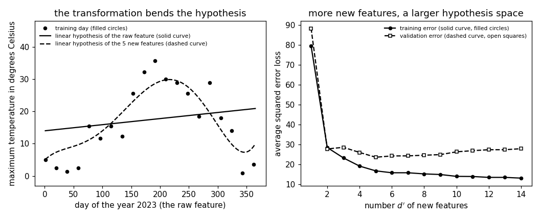
Numerical companion to the glossary entry 'featuretransformation'. Each data point is one day; its single raw feature is the day of the year, rescaled to the interval [-1, 1], and its label is the maximum daytime temperature. A linear hypothesis of the raw feature is learned by least squares on the 365 days of 2023 (the training set) and judged on the 366 days of 2024 (the validation set). The same method is then applied to the transformed feature vector (x, x^2, ..., x^(d')), so that a linear hypothesis on the new features is a polynomial of the raw one. The demo recomputes the three numbers the entry states: the error of the straight line, the error after the transformation with d' = 5 new features, and the training and validation error over d' = 1, ..., 14, where the training error keeps falling while the validation error turns up.
Run it without installing anything:uv run https://dictionaryofml.org/terms/featuretransformation.py
uv downloads this script and the pinned NumPy and Matplotlib it needs, then runs it; the script fetches any input file it uses. To keep the output files, download featuretransformation.py into a folder and run uv run featuretransformation.py there. With NumPy and Matplotlib already installed, python3 featuretransformation.py, from any directory — it writes its output files into the current directory. Fixed seeds, so the printed numbers reproduce exactly. Download featuretransformation.py · Notebook · Open in Colab
Before running a downloaded copy, scan it: uvx bandit -q -t B102,B307,B602,B605 featuretransformation.py (B102,B307,B602,B605 are the exec, eval and shell checks of bandit) reports nothing: the script runs no shell command and evaluates no generated code.
One cell per block of the script: the code, and what that code printed when it last ran here
"""A feature transformation on the daily weather at Krems an der Donau
(Austria): a linear hypothesis on the raw feature, and the same method on a
polynomial transformation of it.

Purpose
-------
Numerical companion to the glossary entry 'featuretransformation'.  Each
data point is one day; its single raw feature is the day of the year,
rescaled to the interval [-1, 1], and its label is the maximum daytime
temperature.  A linear hypothesis of the raw feature is learned by least
squares on the 365 days of 2023 (the training set) and judged on the 366
days of 2024 (the validation set).  The same method is then applied to the
transformed feature vector (x, x^2, ..., x^(d')), so that a linear
hypothesis on the new features is a polynomial of the raw one.  The demo
recomputes the three numbers the entry states: the error of the straight
line, the error after the transformation with d' = 5 new features, and the
training and validation error over d' = 1, ..., 14, where the training
error keeps falling while the validation error turns up.

It also shows that the number of new features is not the whole choice:
the three odd powers x, x^3, x^5 leave the validation error above that of
predicting the sample mean of the training labels, while the two even
powers x^2, x^4 alone are better than all five powers together, because
the seasonal cycle is nearly symmetric about the middle of the year.

It verifies the composition claim twice: the two-step evaluation
(transform the raw feature, then apply the linear hypothesis) agrees with
the polynomial evaluated directly, and the composed hypothesis is not an
affine function of the raw feature, while the one learned on the raw
feature is.

Self-contained (numpy and matplotlib only), fixed seeds; the GeoSphere
download falls back to the committed CSV.

Blocks
------
[B-data]  Daily maximum temperature at Krems for 2023 and 2024 (731 days,
          no missing value), the raw feature and the label.
[B-raw]   A linear hypothesis of the raw feature, learned by least squares
          on the 2023 days; its training and validation error against the
          error of predicting the sample mean of the training labels.
[B-trafo] The polynomial feature transformation with d' = 5 new features;
          the training and validation error of a linear hypothesis on the
          new features, and the two composition checks.
[B-prune] Training and validation error over d' = 1, ..., 14: the training
          error falls with d', the validation error is smallest at d' = 5
          and rises beyond it.
[B-blind] A transformation fixed in advance can discard what the label
          depends on: the three odd powers of the raw feature against the
          two even ones, and the symmetry of the seasonal cycle about the
          middle of the year that separates them.
[B-draw]  The thinned set of 20 training days drawn in the figure, the
          plot CSVs, and the matplotlib preview.

Outputs
-------
featuretransformation_weather.csv    : date, tmax for 2023 and 2024
                                       (committed copy of the download).
featuretransformation_days_plot.csv  : every 19th day of 2023, 20 of the
                                       365, for the plot of panel (a).
featuretransformation_curves.csv     : the two learned hypotheses on a grid
                                       of days, d' = 1 and d' = 5.
featuretransformation_errors.csv     : d', training error, validation error.
featuretransformation.png            : matplotlib preview (checking only).
"""

# /// script
# requires-python = ">=3.10"
# dependencies = ["matplotlib==3.10.7", "numpy==2.3.4"]
# ///

import json
import urllib.request
from pathlib import Path

import numpy as np
import matplotlib

matplotlib.use("Agg")
import matplotlib.pyplot as plt

OUT_DIR = Path(__file__).parent

DPRIME_MAX = 14          # largest number of new features examined
DPRIME_STAR = 5          # the number of new features the entry reports
THIN = 19                # every 19th training day is drawn

report = []


def check(name, ok):
    report.append((name, bool(ok)))
    print(f"  [{'ok' if ok else 'FAIL'}] {name}")
Installed 11 packages in 61ms
Daily maximum temperature at Krems for 2023 and 2024 (731 days, no missing value), the raw feature and the label.
print("[B-data] daily maximum temperature at Krems, 2023 and 2024")
URL = ("https://dataset.api.hub.geosphere.at/v1/station/historical/"
       "klima-v2-1d?parameters=tlmax&station_ids=3805"
       "&start=2023-01-01&end=2024-12-31")
CSV = OUT_DIR / "featuretransformation_weather.csv"
try:
    with urllib.request.urlopen(URL, timeout=120) as resp:
        payload = json.load(resp)
    params = payload["features"][0]["properties"]["parameters"]
    records = [(stamp[:10], hi)
               for stamp, hi in zip(payload["timestamps"],
                                    params["tlmax"]["data"])]
    with open(CSV, "w") as fh:
        fh.write("date,tmax\n")
        for day, hi in records:
            fh.write(f"{day},{hi}\n")
    print(f"    downloaded {len(records)} days")
except OSError as err:
    print(f"    download failed ({err}); reading the committed CSV")
    rows = CSV.read_text().strip().splitlines()[1:]
    records = [(d, float(v)) for d, v in (r.split(",") for r in rows)]

check("[B-data] 731 days for 2023 and 2024", len(records) == 731)
check("[B-data] no day is missing its maximum temperature",
      all(hi is not None for _, hi in records))

y_all = np.array([float(hi) for _, hi in records])
is23 = np.array([d.startswith("2023") for d, _ in records])
y_tr, y_va = y_all[is23], y_all[~is23]
m_tr, m_va = len(y_tr), len(y_va)
# the raw feature of a day: its position in the year, rescaled to [-1, 1]
day_tr = np.arange(1, m_tr + 1)
day_va = np.arange(1, m_va + 1)
x_tr = 2.0 * day_tr / m_tr - 1.0
x_va = 2.0 * day_va / m_va - 1.0
check(f"[B-data] the raw feature of a training day runs from "
      f"{x_tr[0]:.4f} to {x_tr[-1]:.4f}; {m_tr} training days and "
      f"{m_va} validation days",
      -1.0 < x_tr[0] < -0.99 and abs(x_tr[-1] - 1.0) < 1e-12)


def learn(dprime):
    """Least squares on the transformed training features; returns the
    weight vector of the linear hypothesis on the d' new features."""
    A = np.vander(x_tr, dprime + 1, increasing=True)
    return np.linalg.lstsq(A, y_tr, rcond=None)[0]


def errors(w):
    """Training and validation error (average squared error loss)."""
    dprime = len(w) - 1
    tr = np.mean((y_tr - np.vander(x_tr, dprime + 1, increasing=True) @ w) ** 2)
    va = np.mean((y_va - np.vander(x_va, dprime + 1, increasing=True) @ w) ** 2)
    return float(tr), float(va)
[B-data] daily maximum temperature at Krems, 2023 and 2024
    downloaded 731 days
  [ok] [B-data] 731 days for 2023 and 2024
  [ok] [B-data] no day is missing its maximum temperature
  [ok] [B-data] the raw feature of a training day runs from -0.9945 to 1.0000; 365 training days and 366 validation days
A linear hypothesis of the raw feature, learned by least squares on the 2023 days; its training and validation error against the error of predicting the sample mean of the training labels.
print("[B-raw] a linear hypothesis of the raw feature alone")
w_raw = learn(1)
tr_raw, va_raw = errors(w_raw)
mean_tr = float(np.mean(y_tr))
va_mean = float(np.mean((y_va - mean_tr) ** 2))
span = float(y_tr.max() - y_tr.min())
check(f"[B-raw] the learned hypothesis is h(x) = {w_raw[0]:.2f} "
      f"{'+' if w_raw[1] >= 0 else '-'} {abs(w_raw[1]):.2f} x: it rises by "
      f"{2 * abs(w_raw[1]):.1f} degrees from the first to the last day of "
      f"the year, against a label range of {span:.1f} degrees",
      2 * abs(w_raw[1]) < 0.25 * span)
check(f"[B-raw] training error {tr_raw:.2f} and validation error "
      f"{va_raw:.2f} squared degrees", tr_raw > 0 and va_raw > 0)
check(f"[B-raw] predicting the sample mean {mean_tr:.2f} degrees of the "
      f"training labels gives the validation error {va_mean:.2f}, below the "
      f"{va_raw:.2f} of the straight line, so the raw feature is of no use "
      f"to a linear hypothesis", va_raw > va_mean)
[B-raw] a linear hypothesis of the raw feature alone
  [ok] [B-raw] the learned hypothesis is h(x) = 17.43 + 3.45 x: it rises by 6.9 degrees from the first to the last day of the year, against a label range of 38.4 degrees
  [ok] [B-raw] training error 79.43 and validation error 88.22 squared degrees
  [ok] [B-raw] predicting the sample mean 17.44 degrees of the training labels gives the validation error 84.85, below the 88.22 of the straight line, so the raw feature is of no use to a linear hypothesis
The polynomial feature transformation with d' = 5 new features; the training and validation error of a linear hypothesis on the new features, and the two composition checks.
print(f"[B-trafo] a polynomial feature transformation with "
      f"{DPRIME_STAR} new features")
w_star = learn(DPRIME_STAR)
tr_star, va_star = errors(w_star)
check(f"[B-trafo] training error {tr_star:.2f} and validation error "
      f"{va_star:.2f} squared degrees with {DPRIME_STAR} new features",
      va_star < va_raw)
check(f"[B-trafo] the validation error falls from {va_raw:.2f} to "
      f"{va_star:.2f} squared degrees, a factor of "
      f"{va_raw / va_star:.1f}", va_star < va_raw / 3)
# composition, step by step: transform the raw feature, then apply the
# linear hypothesis on the new features
probe = np.array([-0.7, -0.2, 0.0, 0.35, 0.8])
two_step = np.array([float(w_star[0]
                          + np.dot(w_star[1:],
                                   np.array([xx ** j for j in
                                             range(1, DPRIME_STAR + 1)])))
                     for xx in probe])
direct = np.polyval(w_star[::-1], probe)
check(f"[B-trafo] the two-step evaluation (transform, then the linear "
      f"hypothesis) agrees with the polynomial of the raw feature at "
      f"{len(probe)} probe days, largest gap "
      f"{np.max(np.abs(two_step - direct)):.2e}",
      np.allclose(two_step, direct, atol=1e-9))
mid = 0.5 * (probe[0] + probe[-1])
comp_mid = float(np.polyval(w_star[::-1], mid))
comp_avg = 0.5 * (two_step[0] + two_step[-1])
line_mid = float(w_raw[0] + w_raw[1] * mid)
line_avg = 0.5 * ((w_raw[0] + w_raw[1] * probe[0])
                  + (w_raw[0] + w_raw[1] * probe[-1]))
check(f"[B-trafo] the composed hypothesis is not affine in the raw "
      f"feature: at the midpoint of two days it gives {comp_mid:.2f} "
      f"degrees against the average {comp_avg:.2f} of its two values",
      abs(comp_mid - comp_avg) > 1.0)
check(f"[B-trafo] the hypothesis learned on the raw feature is affine: "
      f"{line_mid:.4f} against {line_avg:.4f}",
      abs(line_mid - line_avg) < 1e-9)
[B-trafo] a polynomial feature transformation with 5 new features
  [ok] [B-trafo] training error 16.80 and validation error 23.63 squared degrees with 5 new features
  [ok] [B-trafo] the validation error falls from 88.22 to 23.63 squared degrees, a factor of 3.7
  [ok] [B-trafo] the two-step evaluation (transform, then the linear hypothesis) agrees with the polynomial of the raw feature at 5 probe days, largest gap 1.07e-14
  [ok] [B-trafo] the composed hypothesis is not affine in the raw feature: at the midpoint of two days it gives 28.63 degrees against the average 9.22 of its two values
  [ok] [B-trafo] the hypothesis learned on the raw feature is affine: 17.6022 against 17.6022
Training and validation error over d' = 1, ..., 14: the training error falls with d', the validation error is smallest at d' = 5 and rises beyond it.
print("[B-prune] training and validation error over the number of new "
      "features")
dprimes = np.arange(1, DPRIME_MAX + 1)
tr_curve, va_curve = [], []
for dp in dprimes:
    a, b = errors(learn(int(dp)))
    tr_curve.append(a)
    va_curve.append(b)
tr_curve, va_curve = np.array(tr_curve), np.array(va_curve)
best = int(dprimes[int(np.argmin(va_curve))])
check(f"[B-prune] the training error falls from {tr_curve[0]:.2f} to "
      f"{tr_curve[-1]:.2f} squared degrees as d' grows from 1 to "
      f"{DPRIME_MAX}", np.all(np.diff(tr_curve) < 1e-6))
check(f"[B-prune] the validation error is smallest at d' = {best} with "
      f"{va_curve.min():.2f} squared degrees", best == DPRIME_STAR)
check(f"[B-prune] beyond d' = {best} the validation error rises again, to "
      f"{va_curve[-1]:.2f} at d' = {DPRIME_MAX}, while the training error "
      f"keeps falling", va_curve[-1] > va_curve.min() + 2.0)
check(f"[B-prune] the gap between the two errors widens from "
      f"{va_curve[0] - tr_curve[0]:.2f} at d' = 1 to "
      f"{va_curve[-1] - tr_curve[-1]:.2f} at d' = {DPRIME_MAX}",
      va_curve[-1] - tr_curve[-1] > va_curve[0] - tr_curve[0])
[B-prune] training and validation error over the number of new features
  [ok] [B-prune] the training error falls from 79.43 to 13.15 squared degrees as d' grows from 1 to 14
  [ok] [B-prune] the validation error is smallest at d' = 5 with 23.63 squared degrees
  [ok] [B-prune] beyond d' = 5 the validation error rises again, to 27.91 at d' = 14, while the training error keeps falling
  [ok] [B-prune] the gap between the two errors widens from 8.79 at d' = 1 to 14.76 at d' = 14
A transformation fixed in advance can discard what the label depends on: the three odd powers of the raw feature against the two even ones, and the symmetry of the seasonal cycle about the middle of the year that separates them.
print("[B-blind] a transformation fixed in advance can discard what the "
      "label depends on")


def errors_on(cols_tr, cols_va):
    """Training and validation error of least squares on given columns."""
    A = np.column_stack([np.ones(m_tr)] + cols_tr)
    B = np.column_stack([np.ones(m_va)] + cols_va)
    w = np.linalg.lstsq(A, y_tr, rcond=None)[0]
    return (float(np.mean((y_tr - A @ w) ** 2)),
            float(np.mean((y_va - B @ w) ** 2)))


tr_odd, va_odd = errors_on([x_tr, x_tr ** 3, x_tr ** 5],
                           [x_va, x_va ** 3, x_va ** 5])
tr_even, va_even = errors_on([x_tr ** 2, x_tr ** 4], [x_va ** 2, x_va ** 4])
# the label as a function of the raw feature, split into its symmetric and
# its antisymmetric part about x = 0, the middle of the year; the two parts
# are uncorrelated, so the average squared deviation of the labels from
# their sample mean splits between them
y_mirror = np.interp(-x_tr, x_tr, y_tr)
sym = 0.5 * (y_tr + y_mirror)
anti = 0.5 * (y_tr - y_mirror)
share = float(sym.var() / (sym.var() + anti.var()))
check(f"[B-blind] the average squared deviation "
      f"{sym.var() + anti.var():.2f} of the training labels from their "
      f"sample mean splits between the symmetric and the antisymmetric "
      f"part, and matches the {y_tr.var():.2f} computed directly",
      abs(sym.var() + anti.var() - y_tr.var()) < 1e-9)
check(f"[B-blind] the maximum temperature at Krems is nearly symmetric "
      f"about the middle of the year: {100 * share:.0f} percent of that "
      f"squared deviation sits in the symmetric part", share > 0.7)
check(f"[B-blind] the three odd powers x, x^3, x^5 are antisymmetric about "
      f"the middle of the year and leave the validation error at "
      f"{va_odd:.2f} squared degrees, above the {va_mean:.2f} of the "
      f"constant hypothesis, although they deliver three new features "
      f"where the raw feature is one", va_odd > va_mean)
check(f"[B-blind] the two even powers x^2, x^4 alone give the validation "
      f"error {va_even:.2f} squared degrees, below the {va_star:.2f} of all "
      f"five powers", va_even < va_star)
check(f"[B-blind] the training error separates the two choices as well: "
      f"{tr_odd:.2f} squared degrees for the odd powers against "
      f"{tr_even:.2f} for the even ones", tr_odd > tr_even)
[B-blind] a transformation fixed in advance can discard what the label depends on
  [ok] [B-blind] the average squared deviation 83.40 of the training labels from their sample mean splits between the symmetric and the antisymmetric part, and matches the 83.40 computed directly
  [ok] [B-blind] the maximum temperature at Krems is nearly symmetric about the middle of the year: 77 percent of that squared deviation sits in the symmetric part
  [ok] [B-blind] the three odd powers x, x^3, x^5 are antisymmetric about the middle of the year and leave the validation error at 86.69 squared degrees, above the 84.85 of the constant hypothesis, although they deliver three new features where the raw feature is one
  [ok] [B-blind] the two even powers x^2, x^4 alone give the validation error 21.96 squared degrees, below the 23.63 of all five powers
  [ok] [B-blind] the training error separates the two choices as well: 71.57 squared degrees for the odd powers against 28.75 for the even ones
The thinned set of 20 training days drawn in the figure, the plot CSVs, and the matplotlib preview.
print("[B-draw] the thinned training days, the plot CSVs and the preview")
thin = np.arange(0, m_tr, THIN)
check(f"[B-draw] {len(thin)} of the {m_tr} training days are drawn, "
      f"every {THIN}th in calendar order", len(thin) <= 21)
with open(OUT_DIR / "featuretransformation_days_plot.csv", "w") as fh:
    fh.write("day,tmax\n")
    for i in thin:
        fh.write(f"{day_tr[i]},{y_tr[i]:.1f}\n")
grid_day = np.linspace(1, m_tr, 200)
grid_x = 2.0 * grid_day / m_tr - 1.0
with open(OUT_DIR / "featuretransformation_curves.csv", "w") as fh:
    fh.write("day,raw,poly\n")
    for d, xx in zip(grid_day, grid_x):
        fh.write(f"{d:.3f},{np.polyval(w_raw[::-1], xx):.4f},"
                 f"{np.polyval(w_star[::-1], xx):.4f}\n")
with open(OUT_DIR / "featuretransformation_errors.csv", "w") as fh:
    fh.write("dprime,train,val\n")
    for dp, a, b in zip(dprimes, tr_curve, va_curve):
        fh.write(f"{dp},{a:.4f},{b:.4f}\n")

fig, (ax1, ax2) = plt.subplots(1, 2, figsize=(9.6, 3.9))
ax1.plot(day_tr[thin], y_tr[thin], "ko", ms=4,
         label="training day (filled circles)")
ax1.plot(grid_day, np.polyval(w_raw[::-1], grid_x), "k-",
         label="linear hypothesis of the raw feature (solid curve)")
ax1.plot(grid_day, np.polyval(w_star[::-1], grid_x), "k--",
         label=f"linear hypothesis of the {DPRIME_STAR} new features "
               f"(dashed curve)")
ax1.set_xlabel("day of the year 2023 (the raw feature)")
ax1.set_ylabel("maximum temperature in degrees Celsius")
ax1.set_ylim(-3, 48)
ax1.set_title("the transformation bends the hypothesis")
ax1.legend(frameon=False, fontsize=7, loc="upper left")
ax2.plot(dprimes, tr_curve, "k-o", ms=4,
         label="training error (solid curve, filled circles)")
ax2.plot(dprimes, va_curve, "k--s", ms=4, mfc="white",
         label="validation error (dashed curve, open squares)")
ax2.set_xlabel("number $d'$ of new features")
ax2.set_ylabel("average squared error loss")
ax2.set_title("more new features, a larger hypothesis space")
ax2.legend(frameon=False, fontsize=7)
fig.tight_layout()
fig.savefig(OUT_DIR / "featuretransformation.png", dpi=110)

n_ok = sum(ok for _, ok in report)
print(f"\n{n_ok}/{len(report)} checks pass")
if n_ok != len(report):
    raise SystemExit(1)
[B-draw] the thinned training days, the plot CSVs and the preview
  [ok] [B-draw] 20 of the 365 training days are drawn, every 19th in calendar order

21/21 checks pass
B-draw writes when the script runs