B-plot writes when the script runsDictionary of Applied Machine Learning · linear discriminant analysis (LDA)
Updated on 2026-11-19
Numerical companion to the entry linear discriminant analysis (LDA): it recomputes what the entry states and prints one line per check
Numerical companion to the glossary entry 'lda'. A day at Krems (GeoSphere station 3805) is a data point with the feature vector (morning minimum temperature, maximum daytime temperature) and the label +1 if precipitation was recorded on that day and -1 otherwise. The days of 2020 to 2023 are the training set and the days of 2024 the test set.
Run it without installing anything:uv run https://dictionaryofml.org/terms/lda.py
uv downloads this script and the pinned NumPy and Matplotlib it needs, then runs it; the script fetches any input file it uses. To keep the output files, download lda.py into a folder and run uv run lda.py there. With NumPy and Matplotlib already installed, python3 lda.py, from any directory — it writes its output files into the current directory. Fixed seeds, so the printed numbers reproduce exactly. Download lda.py · Notebook · Open in Colab
Before running a downloaded copy, scan it: uvx bandit -q -t B102,B307,B602,B605 lda.py (B102,B307,B602,B605 are the exec, eval and shell checks of bandit) reports nothing: the script runs no shell command and evaluates no generated code.
One cell per block of the script: the code, and what that code printed when it last ran here
"""Linear discriminant analysis (LDA) against principal component analysis
(PCA) on the days at Krems an der Donau: one direction chosen without the
labels, one chosen with them.

Purpose
-------
Numerical companion to the glossary entry 'lda'.  A day at Krems
(GeoSphere station 3805) is a data point with the feature vector
(morning minimum temperature, maximum daytime temperature) and the label
+1 if precipitation was recorded on that day and -1 otherwise.  The days
of 2020 to 2023 are the training set and the days of 2024 the test set.

The demo checks the entry's claims.  The sample covariance matrix of the
two features is the sum of the within-class and the between-class
scatter matrix, which is the identity that separates the two methods:
PCA maximizes the quadratic form of the sum over unit-norm directions,
LDA the ratio of the two parts.  The first principal direction carries
93 percent of the sample variance and almost none of the label
information, so the Fisher criterion is three hundred times larger along
the LDA direction than along it, and the two directions are 89 degrees
apart; a sweep over all directions confirms that the LDA direction
attains the maximum.  A threshold on the single
LDA feature classifies the days of 2024 better than a threshold on the
single PCA feature, which does not beat predicting the majority label.

Self-contained (numpy and matplotlib only), no random numbers; the
GeoSphere download falls back to the committed CSV.

Blocks
------
[B-data]     Daily minimum and maximum temperature and precipitation at
             Krems for 2020 to 2024 (1827 days, no missing value); the
             label is +1 on a day with precipitation.
[B-pca]      The sample covariance matrix of the two features on the
             training days, its eigenvalues and the first principal
             direction.
[B-scatter]  The within-class and the between-class scatter matrix, and
             the check that they sum to the sample covariance matrix.
[B-lda]      The LDA direction as the solution of a linear system, the
             Fisher criterion along it and along the first principal
             direction, and a sweep over all directions confirming the
             maximum.
[B-classify] A threshold on each of the two single features, chosen on
             the training days, and the accuracy it reaches on the days
             of 2024.
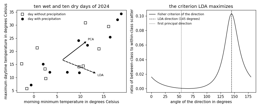
[B-plot]     Twenty of the 366 days of 2024 for the figure, the two
             directions as arrows, and the Fisher criterion against the
             angle of the direction.

Outputs
-------
lda_weather.csv    : date, tmin, tmax, rr for 2020 to 2024 (committed
                     copy, read when the download fails).
lda_wet_plot.csv   : the 10 drawn days of 2024 with precipitation.
lda_dry_plot.csv   : the 10 drawn days of 2024 without precipitation.
lda_axis_pca.csv   : the two endpoints of the arrow along the first
                     principal direction.
lda_axis_lda.csv   : the two endpoints of the arrow along the LDA
                     direction.
lda_fisher.csv     : angle in degrees, Fisher criterion of the direction
                     at that angle.
lda.png            : matplotlib preview (checking only).
"""

# /// script
# requires-python = ">=3.10"
# dependencies = ["matplotlib==3.10.7", "numpy==2.3.4"]
# ///

import json
import urllib.request
from pathlib import Path

import numpy as np
import matplotlib

matplotlib.use("Agg")
import matplotlib.pyplot as plt

OUT_DIR = Path(__file__).parent

report = []


def check(name, ok):
    report.append((name, bool(ok)))
    print(f"  [{'ok' if ok else 'FAIL'}] {name}")


WET = 0.1          # millimetres of precipitation that count as a wet day
                   # (the archive writes -1 for "no precipitation")
Installed 11 packages in 38ms
Daily minimum and maximum temperature and precipitation at Krems for 2020 to 2024 (1827 days, no missing value); the label is +1 on a day with precipitation.
print("[B-data] daily temperatures and precipitation at Krems, 2020 to 2024")
URL = ("https://dataset.api.hub.geosphere.at/v1/station/historical/"
       "klima-v2-1d?parameters=tlmin,tlmax,rr&station_ids=3805"
       "&start=2020-01-01&end=2024-12-31")
CSV = OUT_DIR / "lda_weather.csv"
try:
    with urllib.request.urlopen(URL, timeout=180) as resp:
        payload = json.load(resp)
    par = payload["features"][0]["properties"]["parameters"]
    records = [(stamp[:10], lo, hi, rain)
               for stamp, lo, hi, rain in zip(payload["timestamps"],
                                              par["tlmin"]["data"],
                                              par["tlmax"]["data"],
                                              par["rr"]["data"])]
    with open(CSV, "w") as fh:
        fh.write("date,tmin,tmax,rr\n")
        for day, lo, hi, rain in records:
            fh.write(f"{day},{lo},{hi},{rain}\n")
    print(f"    downloaded {len(records)} days")
except OSError as err:
    print(f"    download failed ({err}); reading the committed CSV")
    rows = CSV.read_text().strip().splitlines()[1:]
    records = [(d, float(a), float(b), float(c))
               for d, a, b, c in (r.split(",") for r in rows)]

check("[B-data] 1827 days for 2020 to 2024", len(records) == 1827)
check("[B-data] no day is missing a measurement",
      all(v is not None for rec in records for v in rec[1:]))
X = np.array([[lo, hi] for _, lo, hi, _ in records])
rr = np.array([rain for _, _, _, rain in records])
y = np.where(rr >= WET, 1.0, -1.0)
year = np.array([int(d[:4]) for d, _, _, _ in records])
tr, te = year <= 2023, year == 2024
check(f"[B-data] {int((y[tr] > 0).sum())} of the {int(tr.sum())} training "
      f"days and {int((y[te] > 0).sum())} of the {int(te.sum())} days of "
      f"2024 carry precipitation",
      tr.sum() == 1461 and te.sum() == 366)
Xtr, ytr, Xte, yte = X[tr], y[tr], X[te], y[te]
m = len(Xtr)
[B-data] daily temperatures and precipitation at Krems, 2020 to 2024
    downloaded 1827 days
  [ok] [B-data] 1827 days for 2020 to 2024
  [ok] [B-data] no day is missing a measurement
  [ok] [B-data] 602 of the 1461 training days and 144 of the 366 days of 2024 carry precipitation
The sample covariance matrix of the two features on the training days, its eigenvalues and the first principal direction.
print("[B-pca] first principal direction of the two features")
mean = Xtr.mean(axis=0)
Xc = Xtr - mean
Q = Xc.T @ Xc / m
lam, U = np.linalg.eigh(Q)              # ascending eigenvalues
lam, U = lam[::-1], U[:, ::-1]
u1 = U[:, 0] * np.sign(U[:, 0].sum())   # point it towards warmer days
check(f"[B-pca] sample mean ({mean[0]:.2f}, {mean[1]:.2f}) degrees; "
      f"eigenvalues {lam[0]:.1f} and {lam[1]:.1f} squared degrees",
      lam[0] > lam[1] > 0)
check(f"[B-pca] the first principal direction ({u1[0]:.3f}, {u1[1]:.3f}) "
      f"carries {100 * lam[0] / lam.sum():.0f} percent of the sample "
      f"variance", lam[0] / lam.sum() > 0.9)
[B-pca] first principal direction of the two features
  [ok] [B-pca] sample mean (6.12, 16.69) degrees; eigenvalues 122.1 and 9.3 squared degrees
  [ok] [B-pca] the first principal direction (0.590, 0.807) carries 93 percent of the sample variance
The within-class and the between-class scatter matrix, and the check that they sum to the sample covariance matrix.
print("[B-scatter] the two scatter matrices and their sum")
mu = {c: Xtr[ytr == c].mean(axis=0) for c in (-1.0, 1.0)}
frac = {c: (ytr == c).mean() for c in (-1.0, 1.0)}
S = sum(((Xtr[ytr == c] - mu[c]).T @ (Xtr[ytr == c] - mu[c])) / m
        for c in (-1.0, 1.0))
B = sum(frac[c] * np.outer(mu[c] - mean, mu[c] - mean) for c in (-1.0, 1.0))
check(f"[B-scatter] class means: dry ({mu[-1.0][0]:.2f}, "
      f"{mu[-1.0][1]:.2f}), wet ({mu[1.0][0]:.2f}, {mu[1.0][1]:.2f}) "
      f"degrees", mu[1.0][0] > mu[-1.0][0])
check("[B-scatter] the within-class and the between-class scatter matrix "
      "sum to the sample covariance matrix", np.allclose(S + B, Q))
check(f"[B-scatter] the between-class scatter has rank 1 and trace "
      f"{np.trace(B):.3f}, against {np.trace(S):.1f} for the within-class "
      f"scatter", np.linalg.matrix_rank(B) == 1)
[B-scatter] the two scatter matrices and their sum
  [ok] [B-scatter] class means: dry (5.39, 17.01), wet (7.16, 16.23) degrees
  [ok] [B-scatter] the within-class and the between-class scatter matrix sum to the sample covariance matrix
  [ok] [B-scatter] the between-class scatter has rank 1 and trace 0.910, against 130.5 for the within-class scatter
The LDA direction as the solution of a linear system, the Fisher criterion along it and along the first principal direction, and a sweep over all directions confirming the maximum.
print("[B-lda] the LDA direction and the Fisher criterion")
w = np.linalg.solve(S, mu[1.0] - mu[-1.0])
w = w / np.linalg.norm(w)


def fisher(d):
    return float((d @ B @ d) / (d @ S @ d))


diff = mu[1.0] - mu[-1.0]
check(f"[B-lda] the LDA direction ({w[0]:.3f}, {w[1]:.3f}) is the "
      f"direction that the within-class scatter maps onto the difference "
      f"of the two class means",
      abs((S @ w)[0] * diff[1] - (S @ w)[1] * diff[0]) < 1e-12
      and (S @ w) @ diff > 0)
check(f"[B-lda] Fisher criterion {fisher(w):.4f} along the LDA direction "
      f"against {fisher(u1):.5f} along the first principal direction, a "
      f"factor of {fisher(w) / fisher(u1):.0f}", fisher(w) > 50 * fisher(u1))
ang = np.arange(0.0, 180.0, 0.05)
J = np.array([fisher(np.array([np.cos(np.deg2rad(a)), np.sin(np.deg2rad(a))]))
              for a in ang])
best = ang[int(np.argmax(J))]
w_ang = np.rad2deg(np.arctan2(w[1], w[0])) % 180.0
check(f"[B-lda] a sweep over all directions peaks at {best:.2f} degrees, "
      f"the angle {w_ang:.2f} degrees of the LDA direction",
      abs(best - w_ang) < 0.1 and abs(J.max() - fisher(w)) < 1e-6)
check(f"[B-lda] the LDA direction weighs the two features with opposite "
      f"signs, so its feature falls with the daily temperature range; "
      f"its angle to the first principal direction is "
      f"{np.rad2deg(np.arccos(abs(w @ u1))):.0f} degrees", w[0] * w[1] < 0)
[B-lda] the LDA direction and the Fisher criterion
  [ok] [B-lda] the LDA direction (0.817, -0.577) is the direction that the within-class scatter maps onto the difference of the two class means
  [ok] [B-lda] Fisher criterion 0.1031 along the LDA direction against 0.00034 along the first principal direction, a factor of 303
  [ok] [B-lda] a sweep over all directions peaks at 144.80 degrees, the angle 144.79 degrees of the LDA direction
  [ok] [B-lda] the LDA direction weighs the two features with opposite signs, so its feature falls with the daily temperature range; its angle to the first principal direction is 89 degrees
A threshold on each of the two single features, chosen on the training days, and the accuracy it reaches on the days of 2024.
print("[B-classify] a threshold on each of the two single features")


def best_threshold(scores, labels):
    cand = np.unique(scores)
    cand = np.concatenate([[cand[0] - 1.0], (cand[:-1] + cand[1:]) / 2])
    acc = [max(((np.where(scores > t, 1.0, -1.0) == labels).mean(),
                ((np.where(scores > t, -1.0, 1.0) == labels).mean()))
               ) for t in cand]
    i = int(np.argmax(acc))
    hi = (np.where(cand[i] < scores, 1.0, -1.0) == labels).mean() >= acc[i]
    return float(cand[i]), bool(hi), float(acc[i])


base = max((yte == 1.0).mean(), (yte == -1.0).mean())
res = {}
for tag, d in (("LDA", w), ("PCA", u1)):
    t, hi, acc_tr = best_threshold(Xtr @ d, ytr)
    pred = np.where(Xte @ d > t, 1.0, -1.0) if hi else \
        np.where(Xte @ d > t, -1.0, 1.0)
    res[tag] = float((pred == yte).mean())
    check(f"[B-classify] threshold {t:.2f} on the {tag} feature: accuracy "
          f"{acc_tr:.3f} on the training days, {res[tag]:.3f} on the days "
          f"of 2024", 0.0 < res[tag] < 1.0)
check(f"[B-classify] predicting the majority label reaches {base:.3f} on "
      f"the days of 2024, so the PCA feature gains "
      f"{100 * (res['PCA'] - base):+.1f} and the LDA feature "
      f"{100 * (res['LDA'] - base):+.1f} percentage points",
      res["LDA"] - base > 0.02 > res["PCA"] - base)
[B-classify] a threshold on each of the two single features
  [ok] [B-classify] threshold -3.03 on the LDA feature: accuracy 0.655 on the training days, 0.637 on the days of 2024
  [ok] [B-classify] threshold 36.21 on the PCA feature: accuracy 0.593 on the training days, 0.609 on the days of 2024
  [ok] [B-classify] predicting the majority label reaches 0.607 on the days of 2024, so the PCA feature gains +0.3 and the LDA feature +3.0 percentage points
Twenty of the 366 days of 2024 for the figure, the two directions as arrows, and the Fisher criterion against the angle of the direction.
print("[B-plot] twenty drawn days, the two arrows, the criterion curve")
wet_idx = np.where(yte > 0)[0]
dry_idx = np.where(yte < 0)[0]
step = {"wet": len(wet_idx) // 10, "dry": len(dry_idx) // 10}
draw = {"wet": wet_idx[::step["wet"]][:10], "dry": dry_idx[::step["dry"]][:10]}
check(f"[B-plot] one of every {step['wet']} of the {len(wet_idx)} wet days "
      f"and one of every {step['dry']} of the {len(dry_idx)} dry days of "
      f"2024 are drawn, ten of each",
      len(draw["wet"]) == len(draw["dry"]) == 10)
for tag, idx in draw.items():
    with open(OUT_DIR / f"lda_{tag}_plot.csv", "w") as fh:
        fh.write("x1,x2\n")
        for i in idx:
            fh.write(f"{Xte[i, 0]:.1f},{Xte[i, 1]:.1f}\n")
LEN = 9.0                               # arrow length in degrees
for tag, d in (("pca", u1), ("lda", w)):
    with open(OUT_DIR / f"lda_axis_{tag}.csv", "w") as fh:
        fh.write("x1,x2\n")
        fh.write(f"{mean[0]:.3f},{mean[1]:.3f}\n")
        fh.write(f"{mean[0] + LEN * d[0]:.3f},{mean[1] + LEN * d[1]:.3f}\n")
    print(f"    arrow {tag}: tip at ({mean[0] + LEN * d[0]:.2f}, "
          f"{mean[1] + LEN * d[1]:.2f})")
with open(OUT_DIR / "lda_fisher.csv", "w") as fh:
    fh.write("angle,J\n")
    for a, j in zip(ang[::20], J[::20]):
        fh.write(f"{a:.2f},{j:.5f}\n")
print(f"    criterion curve: {len(ang[::20])} angles, maximum "
      f"{J.max():.4f} at {best:.2f} degrees, minimum {J.min():.5f}")

fig, (ax1, ax2) = plt.subplots(1, 2, figsize=(9.6, 4.0))
ax1.plot(Xte[draw["dry"], 0], Xte[draw["dry"], 1], "s", mfc="none",
         mec="black", label="day without precipitation")
ax1.plot(Xte[draw["wet"], 0], Xte[draw["wet"], 1], "o", color="black",
         label="day with precipitation")
ax1.annotate("", xy=mean + LEN * u1, xytext=mean,
             arrowprops=dict(arrowstyle="->", color="black", lw=1.6))
ax1.annotate("", xy=mean + LEN * w, xytext=mean,
             arrowprops=dict(arrowstyle="->", color="black", lw=1.6, ls="--"))
ax1.text(*(mean + LEN * u1), " PCA", va="bottom", fontsize=8)
ax1.text(*(mean + LEN * w), " LDA", va="top", fontsize=8)
ax1.set_xlabel("morning minimum temperature in degrees Celsius")
ax1.set_ylabel("maximum daytime temperature in degrees Celsius")
ax1.set_title("ten wet and ten dry days of 2024")
ax1.legend(frameon=False, fontsize=8, loc="upper left")
ax2.plot(ang, J, "k-", lw=1.0, label="Fisher criterion of the direction")
ax2.axvline(w_ang, color="black", ls="--", lw=0.9,
            label=f"LDA direction ({w_ang:.0f} degrees)")
ax2.axvline(np.rad2deg(np.arctan2(u1[1], u1[0])) % 180.0, color="black",
            ls=":", lw=0.9, label="first principal direction")
ax2.set_xlabel("angle of the direction in degrees")
ax2.set_ylabel("ratio of between-class to within-class scatter")
ax2.set_title("the criterion LDA maximizes")
ax2.legend(frameon=False, fontsize=8)
fig.tight_layout()
fig.savefig(OUT_DIR / "lda.png", dpi=110)

n_ok = sum(ok for _, ok in report)
print(f"\n{n_ok}/{len(report)} checks pass")
if n_ok != len(report):
    raise SystemExit(1)
[B-plot] twenty drawn days, the two arrows, the criterion curve
  [ok] [B-plot] one of every 14 of the 144 wet days and one of every 22 of the 222 dry days of 2024 are drawn, ten of each
    arrow pca: tip at (11.43, 23.95)
    arrow lda: tip at (13.47, 11.50)
    criterion curve: 180 angles, maximum 0.1031 at 144.80 degrees, minimum 0.00000

16/16 checks pass
B-plot writes when the script runs