eigenvector.py, which recomputes what the entry states: the script block by block · open in ColabDictionary of Applied Machine Learning: 147 machine-learning terms, each with a definition, a figure, citations and a Python demo · All terms · Demos · Start here
Updated on 2026-11-19
Readiness 90/100
See also eigenvalue eigenvalue decomposition matrix principal component analysis dimensionality reduction
An eigenvector of a square matrix ${\mathbf A}$ is a nonzero vector ${\mathbf x}$ that ${\mathbf A}$ maps to a multiple of itself, ${\mathbf A} {\mathbf x} = \lambda {\mathbf x}$. The number $\lambda$ is the eigenvalue belonging to ${\mathbf x}$, so multiplying by ${\mathbf A}$ keeps ${\mathbf x}$ on the line it spans and only rescales it. An eigenvector is determined only up to a nonzero factor: the eigenvectors belonging to one eigenvalue, together with the zero vector, form the nullspace of ${\mathbf A} - \lambda \mathbf{I}$, a subspace of $\mathbb{R}^{d}$. For a symmetric matrix, the eigenvectors can be chosen to form an orthonormal basis, and collecting them as the columns of one matrix gives the eigenvalue decomposition (EVD). The eigenvectors of the sample covariance matrix of a dataset are the directions that principal component analysis (PCA) keeps and discards. Keeping those belonging to the largest eigenvalues leaves a reconstruction error equal to the sum of the eigenvalues left out.
eigenvector.py, which recomputes what the entry states: the script block by block · open in ColabB-dataEvery day of 2024 at the weather
station Krems an der Donau (Austria) is a data point whose
two features are the lowest and the highest temperature
of that day in degrees Celsius. The sample covariance matrix
$\widehat{{\mathbf C}} \in \mathbb{R}^{2 \times 2}$ of these
$m = 366$ days sends most directions of the plane to a
different direction. Two directions are exceptions: the
matrix returns each of them rescaled and otherwise
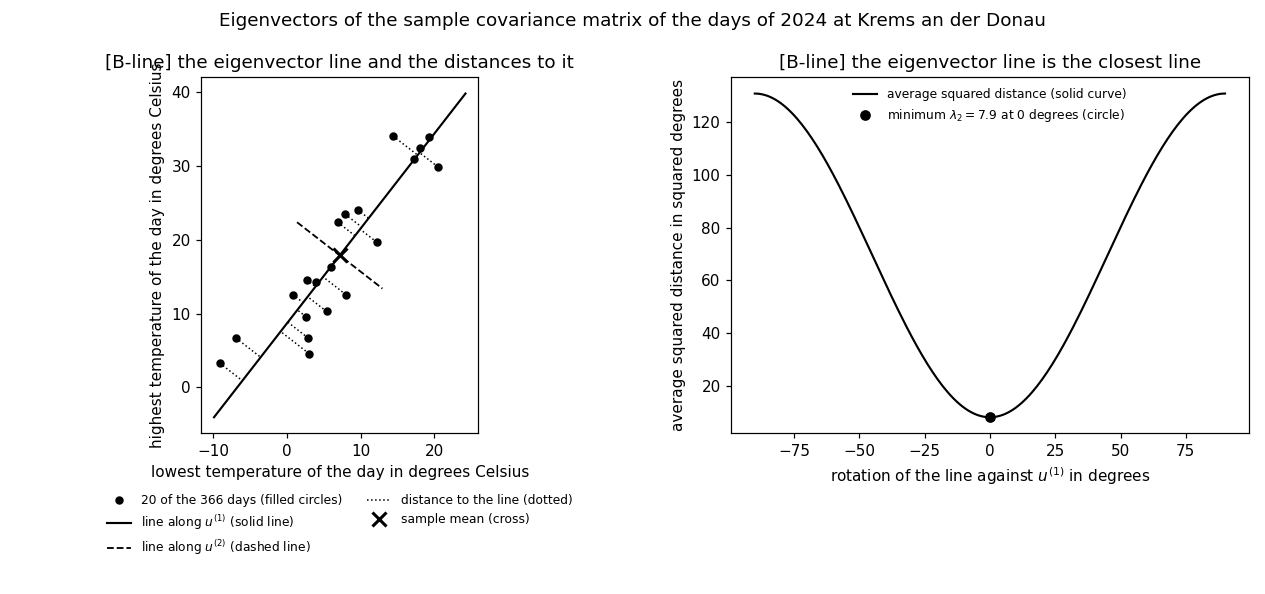
unchanged, and these two are its eigenvectors. The days scatter
most widely along the line spanned by the eigenvector with the
larger scaling factor, and
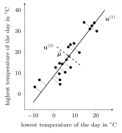
Fig. 1 draws that line through
the sample mean of the days together with the distance of
each drawn day from it.
pythondemos/eigenvector.py
B-eigenspaceAn eigenvector is determined only up to a nonzero factor: when ${\mathbf x}$ satisfies the defining equation \(\eqref{equ_eigenvector_defining_dict}\), so does $c {\mathbf x}$ for every nonzero $c \in \mathbb{R}$, with the same $\lambda$. The eigenvectors belonging to one eigenvalue $\lambda$, together with the zero vector, form the eigenspace of ${\mathbf A}$ for $\lambda$, which is the nullspace of ${\mathbf A} - \lambda \mathbf{I}$ and therefore a subspace of $\mathbb{R}^{d}$ (Horn and Johnson, 2013, Def. 1.4.2). Here, $\mathbf{I}$ is the identity matrix. Each eigenspace of the sample covariance matrix at Krems is a line through the origin, while the matrix $2 \mathbf{I}$ has the single eigenvalue $2$, whose eigenspace is the whole plane. An implementation therefore returns eigenvectors of unit norm, and even then their sign stays arbitrary.
B-orthogonalSymmetry restricts the eigenvectors further. For a real symmetric matrix, every eigenvalue is real and the eigenvectors can be chosen to form an orthonormal basis of $\mathbb{R}^{d}$ (Horn and Johnson, 2013, Thm. 4.1.5; Strang, 2016, Sect. 6.4). Collecting such a basis as the columns of one matrix gives the eigenvalue decomposition (EVD) of the symmetric matrix, which is then a spectral decomposition. The sample covariance matrix $\widehat{{\mathbf C}}$ is symmetric, which is why the two lines of Fig. 1 meet at a right angle. Without symmetry the eigenvectors need not be orthogonal: the matrix with rows $(1.3, 0.8)$ and $(0.4, 0.9)$ has the eigenvectors $(2, 1)^{\top}$ and $(-1, 1)^{\top}$, whose inner product is $-1$.
B-lineEigenvectors are what principal component analysis (PCA) computes. PCA, a method for dimensionality reduction, replaces the $d$ features of a data point by $d' < d$ numbers, chosen so that a linear map rebuilds the feature vector from them with the smallest average squared error loss over a dataset. That reconstruction error is the empirical risk of an instance of empirical risk minimization (ERM), and the eigenvectors of the sample covariance matrix belonging to its $d'$ largest eigenvalues attain its minimum, which equals the sum of the eigenvalues left out (Bishop, 2006, Sect. 12.1.2). For the two temperatures at Krems with $d' = 1$, the retained direction is the eigenvector $\mathbf{u}^{(1)}$ drawn in Fig. 1 and the discarded eigenvalue is $\lambda_{2} = 7.9$ squared degrees, the average squared length of the dotted segments over all $366$ days. The two eigenvalues add up to $138.9$ squared degrees, so the retained direction keeps all but $5.7$ percent of that total, while a line through the sample mean turned by $30$ degrees away from $\mathbf{u}^{(1)}$ would leave $38.7$ squared degrees behind.
See also: eigenvalue, eigenvalue decomposition, spectral decomposition, matrix, vector, nullspace, subspace, symmetric matrix, orthonormal, basis, linear map, sample covariance matrix, principal component analysis, dimensionality reduction.
@misc{dictml_eigenvector,
  author = {Jung, Alexander},
  editor = {Olioumtsevits, Konstantina and Schnoor, Ekkehard},
  title = {eigenvector},
  howpublished = {Dictionary of Applied Machine Learning (course edition)},
  year = {2026},
  doi = {10.5281/zenodo.21569296},
  note = {ISBN 978-952-64-3013-3, CC BY 4.0, retrieved 2026-11-20},
  url = {https://dictionaryofml.org/terms/eigenvector.html}
}