B-line writes when the script runsDictionary of Applied Machine Learning · eigenvector
Updated on 2026-11-19
Numerical companion to the entry eigenvector: it recomputes what the entry states and prints one line per check
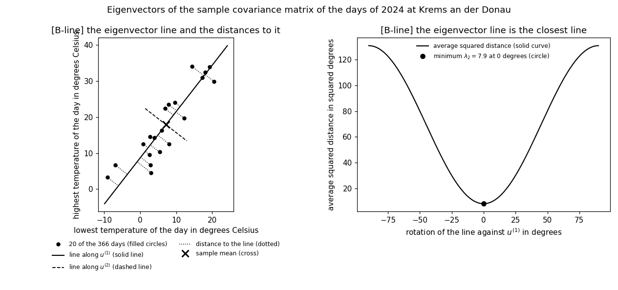
Numerical companion to the glossary entry 'eigenvector'. Each day of 2024 at the GeoSphere Austria weather station Krems an der Donau (station id 3805) is a data point with two features, its lowest and its highest temperature in degrees Celsius. The demo computes the sample covariance matrix C of these days, verifies the defining equation C u = lambda u for its two eigenvectors, shows that an eigenvector is determined only up to a nonzero factor (the eigenspace is the nullspace of C - lambda I), checks that the eigenvectors of the symmetric C are orthogonal while those of a non-symmetric matrix need not be, and confirms the claim the entry's figure makes: the average squared distance of the days from the line through the sample mean along the leading eigenvector equals the other eigenvalue.
Run it without installing anything:uv run https://dictionaryofml.org/terms/eigenvector.py
uv downloads this script and the pinned NumPy and Matplotlib it needs, then runs it; the script fetches any input file it uses. To keep the output files, download eigenvector.py into a folder and run uv run eigenvector.py there. With NumPy and Matplotlib already installed, python3 eigenvector.py, from any directory — it writes its output files into the current directory. Fixed seeds, so the printed numbers reproduce exactly. Download eigenvector.py · Notebook · Open in Colab
Before running a downloaded copy, scan it: uvx bandit -q -t B102,B307,B602,B605 eigenvector.py (B102,B307,B602,B605 are the exec, eval and shell checks of bandit) reports nothing: the script runs no shell command and evaluates no generated code.
One cell per block of the script: the code, and what that code printed when it last ran here
"""The eigenvectors of the sample covariance matrix of the daily
temperatures at Krems an der Donau: the two directions that the matrix only
rescales, and the line that leaves the smallest average squared distance.

Purpose
-------
Numerical companion to the glossary entry 'eigenvector'.  Each day of 2024
at the GeoSphere Austria weather station Krems an der Donau (station id
3805) is a data point with two features, its lowest and its highest
temperature in degrees Celsius.  The demo computes the sample covariance
matrix C of these days, verifies the defining equation C u = lambda u for
its two eigenvectors, shows that an eigenvector is determined only up to a
nonzero factor (the eigenspace is the nullspace of C - lambda I), checks
that the eigenvectors of the symmetric C are orthogonal while those of a
non-symmetric matrix need not be, and confirms the claim the entry's figure
makes: the average squared distance of the days from the line through the
sample mean along the leading eigenvector equals the other eigenvalue.

Self-contained (numpy and matplotlib only), fixed seed; the GeoSphere
download falls back to the committed CSV.

Blocks
------
[B-data]       Daily lowest and highest temperature at Krems for 2024 (366
               days, no missing value) and their sample covariance matrix.
[B-def]        The defining equation C u = lambda u for the two
               eigenvectors of C, with eigenvalues 130.9 and 7.9 squared
               degrees.
[B-eigenspace] An eigenvector is determined only up to a nonzero factor:
               rescaling one gives an eigenvector with the same eigenvalue,
               and the eigenvectors belonging to one eigenvalue together
               with the zero vector are the nullspace of C - lambda I.  For
               the matrix 2 I every nonzero vector is an eigenvector, so
               that nullspace is the whole plane.
[B-orthogonal] The eigenvectors of the symmetric C are orthogonal and are
               returned with unit norm, while the eigenvectors of the
               non-symmetric matrix [[1.3, 0.8], [0.4, 0.9]] are not
               orthogonal.
[B-line]       The average squared distance of the 366 days from the line
               through the sample mean along the leading eigenvector equals
               the smaller eigenvalue; a line rotated away from that
               eigenvector leaves a larger average.  Writes the CSV files
               of the entry's figure.

Outputs
-------
eigenvector_weather.csv    : date, lowest and highest temperature of each
                             day of 2024 (committed copy).
eigenvector_points.csv     : the 366 days as points (x1 = lowest,
                             x2 = highest temperature, degrees Celsius).
eigenvector_points_plot.csv: every 19th of those days, the 20 drawn in the
                             entry's figure.
eigenvector_line1.csv      : the line through the sample mean along the
                             leading eigenvector, as two endpoints.
eigenvector_line2.csv      : the line through the sample mean along the
                             second eigenvector, as two endpoints.
eigenvector_residuals.csv  : the 20 distance segments of the drawn days
                             from the first line, separated by nan rows.
eigenvector_rotated.csv    : the average squared distance from a line
                             rotated by an angle against the leading
                             eigenvector, over 181 angles.
eigenvector.png            : matplotlib preview (checking only).

Data generated by pythondemos/eigenvector.py.
"""

# /// script
# requires-python = ">=3.10"
# dependencies = ["matplotlib==3.10.7", "numpy==2.3.4"]
# ///

import json
import urllib.request
from pathlib import Path

import numpy as np
import matplotlib

matplotlib.use("Agg")
import matplotlib.pyplot as plt

OUT_DIR = Path(__file__).parent

rng = np.random.default_rng(42)
report = []


def check(name, ok):
    report.append((name, bool(ok)))
    print(f"  [{'ok' if ok else 'FAIL'}] {name}")
Installed 11 packages in 65ms
Daily lowest and highest temperature at Krems for 2024 (366 days, no missing value) and their sample covariance matrix.
print("[B-data] daily lowest and highest temperature at Krems, 2024")
PARAMS = ["tlmin", "tlmax"]
URL = ("https://dataset.api.hub.geosphere.at/v1/station/historical/"
       f"klima-v2-1d?parameters={','.join(PARAMS)}&station_ids=3805"
       "&start=2024-01-01&end=2024-12-31")
CSV = OUT_DIR / "eigenvector_weather.csv"
try:
    with urllib.request.urlopen(URL, timeout=120) as resp:
        payload = json.load(resp)
    params = payload["features"][0]["properties"]["parameters"]
    stamps = [stamp[:10] for stamp in payload["timestamps"]]
    X = np.stack([np.array(params[p]["data"], dtype=float) for p in PARAMS], 1)
    with open(CSV, "w") as fh:
        fh.write("date," + ",".join(PARAMS) + "\n")
        for day, row in zip(stamps, X):
            fh.write(day + "," + ",".join(f"{v:g}" for v in row) + "\n")
    print(f"    downloaded {len(X)} days")
except (OSError, KeyError, ValueError) as err:
    print(f"    download failed ({err}); reading {CSV.name}")
    rows = np.genfromtxt(CSV, delimiter=",", skip_header=1, dtype=str)
    stamps = [str(s) for s in rows[:, 0]]
    X = rows[:, 1:].astype(float)

m = len(X)
check("[B-data] 366 days, each with its lowest and its highest temperature",
      X.shape == (366, 2))
check("[B-data] no day is missing a temperature", bool(np.all(np.isfinite(X))))
check("[B-data] the record matches the archive (Feb 1: -3.8 to 10.4 degrees)",
      stamps[31] == "2024-02-01" and bool(np.allclose(X[31], [-3.8, 10.4])))
mu = X.mean(axis=0)
C = (X - mu).T @ (X - mu) / m
check(f"[B-data] sample mean ({mu[0]:.1f}, {mu[1]:.1f}) degrees; the sample "
      "covariance matrix is symmetric", bool(np.allclose(C, C.T)))
print(f"    C = [[{C[0, 0]:.1f}, {C[0, 1]:.1f}], [{C[1, 0]:.1f}, "
      f"{C[1, 1]:.1f}]] squared degrees")
[B-data] daily lowest and highest temperature at Krems, 2024
    downloaded 366 days
  [ok] [B-data] 366 days, each with its lowest and its highest temperature
  [ok] [B-data] no day is missing a temperature
  [ok] [B-data] the record matches the archive (Feb 1: -3.8 to 10.4 degrees)
  [ok] [B-data] sample mean (7.2, 17.9) degrees; the sample covariance matrix is symmetric
    C = [[54.2, 59.6], [59.6, 84.6]] squared degrees
The defining equation C u = lambda u for the two eigenvectors of C, with eigenvalues 130.9 and 7.9 squared degrees.
print("[B-def] the defining equation C u = lambda u")
lam, U = np.linalg.eigh(C)
order = np.argsort(lam)[::-1]                   # largest eigenvalue first
lam, U = lam[order], U[:, order]
for j in (0, 1):                                # the sign of an eigenvector
    if U[0, j] < 0:                             # is arbitrary; fix x1 > 0
        U[:, j] = -U[:, j]
check("[B-def] both eigenvectors satisfy C u = lambda u to within 1e-13",
      all(np.linalg.norm(C @ U[:, j] - lam[j] * U[:, j]) < 1e-13
          for j in (0, 1)))
check(f"[B-def] the eigenvalues are {lam[0]:.1f} and {lam[1]:.1f} squared "
      "degrees", bool(np.allclose(np.round(lam, 1), [130.9, 7.9])))
print(f"    u1 = ({U[0, 0]:.2f}, {U[1, 0]:.2f}), "
      f"u2 = ({U[0, 1]:.2f}, {U[1, 1]:.2f})")
check("[B-def] neither eigenvector is the zero vector",
      all(np.linalg.norm(U[:, j]) > 0.5 for j in (0, 1)))
notan = np.array([1.0, 0.0])                    # a direction C does tilt
check("[B-def] the first coordinate direction is not an eigenvector: "
      f"C e1 = ({(C @ notan)[0]:.1f}, {(C @ notan)[1]:.1f}) is off its line",
      abs((C @ notan)[1]) > 1e-6)
[B-def] the defining equation C u = lambda u
  [ok] [B-def] both eigenvectors satisfy C u = lambda u to within 1e-13
  [ok] [B-def] the eigenvalues are 130.9 and 7.9 squared degrees
    u1 = (0.61, 0.79), u2 = (0.79, -0.61)
  [ok] [B-def] neither eigenvector is the zero vector
  [ok] [B-def] the first coordinate direction is not an eigenvector: C e1 = (54.2, 59.6) is off its line
An eigenvector is determined only up to a nonzero factor: rescaling one gives an eigenvector with the same eigenvalue, and the eigenvectors belonging to one eigenvalue together with the zero vector are the nullspace of C - lambda I. For the matrix 2 I every nonzero vector is an eigenvector, so that nullspace is the whole plane.
print("[B-eigenspace] the eigenspace is the nullspace of C - lambda I")
FACTOR = -3.7
check(f"[B-eigenspace] rescaling u1 by {FACTOR} gives an eigenvector with "
      "the same eigenvalue",
      np.linalg.norm(C @ (FACTOR * U[:, 0]) - lam[0] * (FACTOR * U[:, 0]))
      < 1e-12)
ranks = [np.linalg.matrix_rank(C - lam[j] * np.eye(2)) for j in (0, 1)]
check("[B-eigenspace] C - lambda I has rank 1 for both eigenvalues, so each "
      "eigenspace is a line through the origin", ranks == [1, 1])
check("[B-eigenspace] u2 spans the nullspace of C - lambda_2 I",
      np.linalg.norm((C - lam[1] * np.eye(2)) @ U[:, 1]) < 1e-12)
twice = 2.0 * np.eye(2)                         # repeated eigenvalue 2
probe = rng.normal(size=(5, 2))
check("[B-eigenspace] for 2 I every nonzero vector is an eigenvector with "
      "eigenvalue 2, so the eigenspace is the whole plane",
      np.linalg.matrix_rank(twice - 2.0 * np.eye(2)) == 0
      and bool(np.allclose(probe @ twice.T, 2.0 * probe)))
[B-eigenspace] the eigenspace is the nullspace of C - lambda I
  [ok] [B-eigenspace] rescaling u1 by -3.7 gives an eigenvector with the same eigenvalue
  [ok] [B-eigenspace] C - lambda I has rank 1 for both eigenvalues, so each eigenspace is a line through the origin
  [ok] [B-eigenspace] u2 spans the nullspace of C - lambda_2 I
  [ok] [B-eigenspace] for 2 I every nonzero vector is an eigenvector with eigenvalue 2, so the eigenspace is the whole plane
The eigenvectors of the symmetric C are orthogonal and are returned with unit norm, while the eigenvectors of the non-symmetric matrix [[1.3, 0.8], [0.4, 0.9]] are not orthogonal.
print("[B-orthogonal] orthogonality of the eigenvectors")
check(f"[B-orthogonal] the two eigenvectors of C are orthogonal (inner "
      f"product {U[:, 0] @ U[:, 1]:.1e})", abs(U[:, 0] @ U[:, 1]) < 1e-14)
check("[B-orthogonal] both are returned with unit norm",
      all(abs(np.linalg.norm(U[:, j]) - 1.0) < 1e-14 for j in (0, 1)))
A = np.array([[1.3, 0.8], [0.4, 0.9]])          # not symmetric
a1, a2 = np.array([2.0, 1.0]), np.array([-1.0, 1.0])
check("[B-orthogonal] the non-symmetric matrix [[1.3, 0.8], [0.4, 0.9]] has "
      "the eigenvectors (2, 1) and (-1, 1)",
      np.linalg.norm(A @ a1 - 1.7 * a1) < 1e-12
      and np.linalg.norm(A @ a2 - 0.5 * a2) < 1e-12)
check(f"[B-orthogonal] those two are not orthogonal (inner product "
      f"{a1 @ a2:.0f})", abs(a1 @ a2) > 0.5)
[B-orthogonal] orthogonality of the eigenvectors
  [ok] [B-orthogonal] the two eigenvectors of C are orthogonal (inner product 0.0e+00)
  [ok] [B-orthogonal] both are returned with unit norm
  [ok] [B-orthogonal] the non-symmetric matrix [[1.3, 0.8], [0.4, 0.9]] has the eigenvectors (2, 1) and (-1, 1)
  [ok] [B-orthogonal] those two are not orthogonal (inner product -1)
The average squared distance of the 366 days from the line through the sample mean along the leading eigenvector equals the smaller eigenvalue; a line rotated away from that eigenvector leaves a larger average. Writes the CSV files of the entry's figure.
print("[B-line] the average squared distance from the eigenvector line")
proj = (X - mu) @ U[:, 0]                       # coordinate along u1
foot = mu + proj[:, None] * U[:, 0]             # closest point on the line
dist2 = np.sum((X - foot) ** 2, axis=1)
check(f"[B-line] the average squared distance of the {m} days from the line "
      f"through the sample mean along u1 is {dist2.mean():.1f} squared "
      f"degrees, the eigenvalue {lam[1]:.1f}",
      abs(dist2.mean() - lam[1]) < 1e-10)
check(f"[B-line] the two eigenvalues sum to the total variance "
      f"{np.trace(C):.1f} squared degrees, so the line leaves "
      f"{100 * lam[1] / np.trace(C):.1f} percent of it",
      abs(lam.sum() - np.trace(C)) < 1e-10)
ANGLE = np.deg2rad(30.0)
normal = -np.sin(ANGLE) * U[:, 0] + np.cos(ANGLE) * U[:, 1]
rot2 = (((X - mu) @ normal) ** 2).mean()
check(f"[B-line] a line rotated by 30 degrees against u1 leaves the larger "
      f"average {rot2:.1f} squared degrees", rot2 > lam[1] + 1.0)
angles = np.linspace(-90.0, 90.0, 181)
normals = (-np.sin(np.deg2rad(angles))[:, None] * U[:, 0]
           + np.cos(np.deg2rad(angles))[:, None] * U[:, 1])
sweep = np.einsum("aj,jk,ak->a", normals, C, normals)
check("[B-line] over 181 rotation angles the smallest average squared "
      "distance is attained at 0 degrees, along u1",
      int(np.argmin(sweep)) == 90 and abs(sweep.min() - lam[1]) < 1e-10)
dirs = (np.cos(np.deg2rad(angles))[:, None] * U[:, 0]
        + np.sin(np.deg2rad(angles))[:, None] * U[:, 1])
spread = np.einsum("aj,jk,ak->a", dirs, C, dirs)
check(f"[B-line] the days spread most widely along u1: their average "
      f"squared distance from the sample mean along it is "
      f"{proj.var():.1f} squared degrees, the eigenvalue {lam[0]:.1f} "
      f"and the largest over the 181 directions",
      abs(proj.var() - lam[0]) < 1e-10
      and int(np.argmax(spread)) == 90)

np.savetxt(OUT_DIR / "eigenvector_points.csv", X, delimiter=",",
           header="x1,x2", comments="", fmt="%.1f")
# the entry's figure draws every 19th day, 20 of the 366, so the distance
# segments stay legible; the eigenvectors come from all 366 days
X_plot = X[::19]
check("[B-line] every 19th day gives 20 days for the entry's figure",
      X_plot.shape[0] == 20)
np.savetxt(OUT_DIR / "eigenvector_points_plot.csv", X_plot, delimiter=",",
           header="x1,x2", comments="", fmt="%.1f")
span1 = 1.04 * np.abs(proj).max()
with open(OUT_DIR / "eigenvector_line1.csv", "w") as fh:
    fh.write("x1,x2\n")
    for t in (-span1, span1):
        p = mu + t * U[:, 0]
        fh.write(f"{p[0]:.3f},{p[1]:.3f}\n")
span2 = 2.6 * np.sqrt(lam[1])
with open(OUT_DIR / "eigenvector_line2.csv", "w") as fh:
    fh.write("x1,x2\n")
    for t in (-span2, span2):
        p = mu + t * U[:, 1]
        fh.write(f"{p[0]:.3f},{p[1]:.3f}\n")
foot_plot = foot[::19]
with open(OUT_DIR / "eigenvector_residuals.csv", "w") as fh:
    fh.write("x1,x2\n")
    for point, base in zip(X_plot, foot_plot):
        fh.write(f"{point[0]:.3f},{point[1]:.3f}\n")
        fh.write(f"{base[0]:.3f},{base[1]:.3f}\n")
        fh.write("nan,nan\n")
with open(OUT_DIR / "eigenvector_rotated.csv", "w") as fh:
    fh.write("angle,avgdist2\n")
    for angle, value in zip(angles, sweep):
        fh.write(f"{angle:.1f},{value:.4f}\n")
check("[B-line] the segment file holds 20 segments separated by nan rows",
      sum(1 for line in (OUT_DIR / "eigenvector_residuals.csv")
          .read_text().splitlines() if line == "nan,nan") == 20)

# ------------------------------------------------------------- preview
fig, ax = plt.subplots(1, 2, figsize=(11.5, 5.4),
                       gridspec_kw=dict(width_ratios=[1.25, 1]))
ax[0].plot(X_plot[:, 0], X_plot[:, 1], "o", color="black", ms=4.5,
           label="20 of the 366 days (filled circles)")
line1 = np.array([mu - span1 * U[:, 0], mu + span1 * U[:, 0]])
line2 = np.array([mu - span2 * U[:, 1], mu + span2 * U[:, 1]])
ax[0].plot(line1[:, 0], line1[:, 1], "k-", lw=1.4,
           label="line along $u^{(1)}$ (solid line)")
ax[0].plot(line2[:, 0], line2[:, 1], "k--", lw=1.2,
           label="line along $u^{(2)}$ (dashed line)")
for point, base in zip(X_plot, foot_plot):
    ax[0].plot([point[0], base[0]], [point[1], base[1]], "k:", lw=1.0)
ax[0].plot([], [], "k:", lw=1.0, label="distance to the line (dotted)")
ax[0].plot(mu[0], mu[1], "x", color="black", ms=9, mew=2,
           label="sample mean (cross)")
ax[0].set_aspect("equal")
ax[0].set_xlabel("lowest temperature of the day in degrees Celsius")
ax[0].set_ylabel("highest temperature of the day in degrees Celsius")
ax[0].set_title("[B-line] the eigenvector line and the distances to it")
ax[0].legend(frameon=False, fontsize=8, loc="upper center",
             bbox_to_anchor=(0.5, -0.14), ncol=2)
ax[1].plot(angles, sweep, "k-", lw=1.4,
           label="average squared distance (solid curve)")
ax[1].plot([0.0], [lam[1]], "o", color="black", ms=6,
           label=f"minimum $\\lambda_2 = {lam[1]:.1f}$ at 0 degrees (circle)")
ax[1].set_xlabel("rotation of the line against $u^{(1)}$ in degrees")
ax[1].set_ylabel("average squared distance in squared degrees")
ax[1].set_title("[B-line] the eigenvector line is the closest line")
ax[1].legend(frameon=False, fontsize=8, loc="upper center")
fig.suptitle("Eigenvectors of the sample covariance matrix of the days of "
             "2024 at Krems an der Donau")
fig.tight_layout()
fig.savefig(OUT_DIR / "eigenvector.png", dpi=110)

print(f"\n{sum(ok for _, ok in report)}/{len(report)} checks passed")
assert all(ok for _, ok in report)
[B-line] the average squared distance from the eigenvector line
  [ok] [B-line] the average squared distance of the 366 days from the line through the sample mean along u1 is 7.9 squared degrees, the eigenvalue 7.9
  [ok] [B-line] the two eigenvalues sum to the total variance 138.9 squared degrees, so the line leaves 5.7 percent of it
  [ok] [B-line] a line rotated by 30 degrees against u1 leaves the larger average 38.7 squared degrees
  [ok] [B-line] over 181 rotation angles the smallest average squared distance is attained at 0 degrees, along u1
  [ok] [B-line] the days spread most widely along u1: their average squared distance from the sample mean along it is 130.9 squared degrees, the eigenvalue 130.9 and the largest over the 181 directions
  [ok] [B-line] every 19th day gives 20 days for the entry's figure
  [ok] [B-line] the segment file holds 20 segments separated by nan rows

23/23 checks passed
B-line writes when the script runs