B-plot writes when the script runsDictionary of Applied Machine Learning · multivariate normal distribution
Updated on 2026-11-19
Numerical companion to the entry multivariate normal distribution: it recomputes what the entry states and prints one line per check
Numerical companion to the glossary entry 'mvndist'. The 366 days of 2024 at Krems are data points with the feature vector (morning minimum temperature, maximum daytime temperature). A multivariate normal distribution is fitted to them by maximum likelihood: its mean vector is the sample mean and its covariance matrix the sample covariance matrix (divisor m). The level sets of the probability density function are ellipses centered at the mean vector, with axes along the eigenvectors of the covariance matrix and half-axes proportional to the square roots of its eigenvalues.
Run it without installing anything:uv run https://dictionaryofml.org/terms/mvndist.py
uv downloads this script and the pinned NumPy and Matplotlib it needs, then runs it; the script fetches any input file it uses. To keep the output files, download mvndist.py into a folder and run uv run mvndist.py there. With NumPy and Matplotlib already installed, python3 mvndist.py, from any directory — it writes its output files into the current directory. Fixed seeds, so the printed numbers reproduce exactly. Download mvndist.py · Notebook · Open in Colab
Before running a downloaded copy, scan it: uvx bandit -q -t B102,B307,B602,B605 mvndist.py (B102,B307,B602,B605 are the exec, eval and shell checks of bandit) reports nothing: the script runs no shell command and evaluates no generated code.
One cell per block of the script: the code, and what that code printed when it last ran here
"""The multivariate normal distribution learned from the days of one year
at Krems an der Donau: the maximum likelihood estimate of its mean vector
and covariance matrix, its elliptical level sets, and how many days the
level sets hold against the Gaussian prediction.

Purpose
-------
Numerical companion to the glossary entry 'mvndist'.  The 366 days of
2024 at Krems are data points with the feature vector (morning minimum
temperature, maximum daytime temperature).  A multivariate normal
distribution is fitted to them by maximum likelihood: its mean vector is
the sample mean and its covariance matrix the sample covariance matrix
(divisor m).  The level sets of the probability density function are
ellipses centered at the mean vector, with axes along the eigenvectors
of the covariance matrix and half-axes proportional to the square roots
of its eigenvalues.

The demo checks the entry's claims: the sample mean and the sample
covariance matrix maximize the likelihood; the density integrates to
one and is constant on each ellipse; a Gaussian random vector lies
inside the level set at c = 1 with probability 1 - exp(-1/2) and inside
the level set at c = 2 with probability 1 - exp(-2); the days at Krems
deviate from these fractions, because the seasons spread them along the
major axis more evenly than a Gaussian would; an affine map of a Gaussian
random vector is Gaussian, so the daily temperature range has the mean
and variance the formula predicts; and the conditional distribution of
the maximum given the minimum is Gaussian with the mean of the least
squares line and a variance that does not depend on the minimum.

Deterministic: the Monte Carlo check of the Gaussian fractions draws
with a fixed seed.  Self-contained: numpy + matplotlib only; the
GeoSphere download falls back to the committed CSV.

Blocks
------
[B-data]      Download the daily minimum and maximum temperature of 2024
              at Krems (GeoSphere station 3805) or read the committed
              copy; 366 days, no missing value.
[B-mle]       The sample mean and the sample covariance matrix (divisor
              m) are the maximum likelihood estimates: the average log
              density of the days is largest there.
[B-density]   The probability density function with these parameters
              integrates to one over the plane.
[B-ellipse]   The level sets at c = 1 and c = 2 are ellipses centered at
              the mean vector; their axes are the eigenvectors of the
              covariance matrix, their half-axes c times the square
              roots of the eigenvalues, and the density is constant on
              each of them.
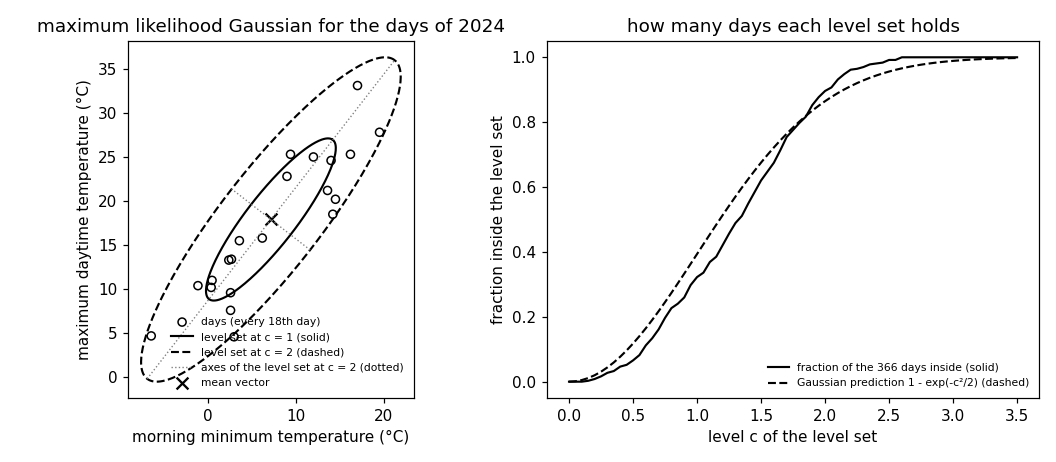
[B-coverage]  Fraction of the 366 days inside the level sets at c = 1,
              2, 3 against the Gaussian prediction 1 - exp(-c^2/2),
              which a Monte Carlo draw from the fitted distribution
              confirms.
[B-linear]    The daily temperature range, an affine map of the feature
              vector, has mean a^T mu and variance a^T C a; the
              conditional distribution of the maximum given the minimum
              has the mean of the least squares line and the variance
              C22 - C12^2 / C11; the range appended as a third feature
              gives a singular covariance matrix.
[B-plot]      Every 18th day for the figure (21 of 366 days), the two
              ellipses with their axes, the mean vector, and the
              coverage curve.

Outputs
-------
mvndist_weather.csv    : date, tmin, tmax (committed copy).
mvndist_days_plot.csv  : the 21 drawn days.
mvndist_mean.csv       : the mean vector, one row.
mvndist_ellipse1.csv   : the level set at c = 1 as a closed polyline.
mvndist_ellipse2.csv   : the level set at c = 2 as a closed polyline.
mvndist_axis1.csv      : the major axis of the level set at c = 2.
mvndist_axis2.csv      : the minor axis of the level set at c = 2.
mvndist_coverage.csv   : c, fraction of the days inside the level set
                         at c, and the Gaussian prediction.
mvndist.png            : matplotlib preview (checking only).
"""

# /// script
# requires-python = ">=3.10"
# dependencies = ["matplotlib==3.10.7", "numpy==2.3.4"]
# ///

import json
import urllib.request
from pathlib import Path

import numpy as np
import matplotlib

matplotlib.use("Agg")
import matplotlib.pyplot as plt

OUT_DIR = Path(__file__).parent
SEED = 20261119

report = []


def check(name, ok):
    report.append((name, bool(ok)))
    print(f"  [{'ok' if ok else 'FAIL'}] {name}")
Download the daily minimum and maximum temperature of 2024 at Krems (GeoSphere station 3805) or read the committed copy; 366 days, no missing value.
print("[B-data] daily minimum and maximum temperature at Krems, 2024")
URL = ("https://dataset.api.hub.geosphere.at/v1/station/historical/"
       "klima-v2-1d?parameters=tlmin,tlmax&station_ids=3805"
       "&start=2024-01-01&end=2024-12-31")
CSV = OUT_DIR / "mvndist_weather.csv"
try:
    with urllib.request.urlopen(URL, timeout=120) as resp:
        payload = json.load(resp)
    params = payload["features"][0]["properties"]["parameters"]
    records = [(stamp[:10], lo, hi)
               for stamp, lo, hi in zip(payload["timestamps"],
                                        params["tlmin"]["data"],
                                        params["tlmax"]["data"])]
    with open(CSV, "w") as fh:
        fh.write("date,tmin,tmax\n")
        for day, lo, hi in records:
            fh.write(f"{day},{lo},{hi}\n")
    print(f"    downloaded {len(records)} days")
except OSError as err:
    print(f"    download failed ({err}); reading the committed CSV")
    rows = CSV.read_text().strip().splitlines()[1:]
    records = [(d, float(a), float(b))
               for d, a, b in (r.split(",") for r in rows)]

check("[B-data] 366 days for 2024", len(records) == 366)
check("[B-data] no day is missing a temperature",
      all(lo is not None and hi is not None for _, lo, hi in records))
X = np.array([[lo, hi] for _, lo, hi in records], dtype=float)
m, d = X.shape


# ---- the probability density function of N(mu, C) on R^d
def log_density(x, mu, C):
    """Logarithm of the density of N(mu, C) at the rows of x."""
    diff = x - mu
    C_inv = np.linalg.inv(C)
    quad = np.einsum("ij,jk,ik->i", diff, C_inv, diff)
    _, logdet = np.linalg.slogdet(C)
    return -0.5 * (d * np.log(2 * np.pi) + logdet + quad)


def mahalanobis_sq(x, mu, C):
    """The quadratic form (x - mu)^T C^{-1} (x - mu) at the rows of x."""
    diff = x - mu
    return np.einsum("ij,jk,ik->i", diff, np.linalg.inv(C), diff)
[B-data] daily minimum and maximum temperature at Krems, 2024
    downloaded 366 days
  [ok] [B-data] 366 days for 2024
  [ok] [B-data] no day is missing a temperature
The sample mean and the sample covariance matrix (divisor m) are the maximum likelihood estimates: the average log density of the days is largest there.
print("[B-mle] maximum likelihood estimates of the mean vector and the "
      "covariance matrix")
mu_hat = X.mean(axis=0)
C_hat = (X - mu_hat).T @ (X - mu_hat) / m
avg_loglik = log_density(X, mu_hat, C_hat).mean()
rng = np.random.default_rng(SEED)
worse = 0
for _ in range(400):
    mu_try = mu_hat + rng.normal(scale=0.5, size=d)
    E = rng.normal(scale=0.08, size=(d, d))
    E = (E + E.T) / 2
    C_try = C_hat + E @ C_hat + C_hat @ E   # a symmetric perturbation
    if np.all(np.linalg.eigvalsh(C_try) > 0):
        worse += log_density(X, mu_try, C_try).mean() < avg_loglik
    else:
        worse += 1
check(f"[B-mle] mean vector ({mu_hat[0]:.1f}, {mu_hat[1]:.1f}) degrees "
      f"Celsius: the sample mean of the {m} days",
      np.allclose(mu_hat, X.sum(axis=0) / m))
check(f"[B-mle] covariance matrix: variances {C_hat[0, 0]:.1f} and "
      f"{C_hat[1, 1]:.1f}, covariance {C_hat[0, 1]:.1f} (squared degrees); "
      f"divisor m, so {m / (m - 1):.4f} times smaller than the unbiased "
      f"version", np.allclose(C_hat, np.cov(X.T, bias=True)))
check(f"[B-mle] the average log density {avg_loglik:.3f} at these "
      f"parameters exceeds it at all 400 perturbed parameter pairs",
      worse == 400)
corr = C_hat[0, 1] / np.sqrt(C_hat[0, 0] * C_hat[1, 1])
check(f"[B-mle] correlation coefficient of minimum and maximum "
      f"temperature {corr:.2f}", 0.8 < corr < 0.95)
[B-mle] maximum likelihood estimates of the mean vector and the covariance matrix
  [ok] [B-mle] mean vector (7.2, 17.9) degrees Celsius: the sample mean of the 366 days
  [ok] [B-mle] covariance matrix: variances 54.2 and 84.6, covariance 59.6 (squared degrees); divisor m, so 1.0027 times smaller than the unbiased version
  [ok] [B-mle] the average log density -6.311 at these parameters exceeds it at all 400 perturbed parameter pairs
  [ok] [B-mle] correlation coefficient of minimum and maximum temperature 0.88
The probability density function with these parameters integrates to one over the plane.
print("[B-density] the probability density function integrates to one")
g1 = np.linspace(mu_hat[0] - 80, mu_hat[0] + 80, 1601)
g2 = np.linspace(mu_hat[1] - 90, mu_hat[1] + 90, 1801)
G1, G2 = np.meshgrid(g1, g2, indexing="ij")
grid = np.column_stack([G1.ravel(), G2.ravel()])
dens = np.exp(log_density(grid, mu_hat, C_hat)).reshape(G1.shape)
integral = np.trapezoid(np.trapezoid(dens, g2, axis=1), g1)
check(f"[B-density] integral over the plane {integral:.5f}",
      abs(integral - 1) < 1e-4)
peak = 1 / (2 * np.pi * np.sqrt(np.linalg.det(C_hat)))
check(f"[B-density] the density is largest at the mean vector, "
      f"{peak:.5f} per squared degree",
      np.isclose(np.exp(log_density(mu_hat[None], mu_hat, C_hat))[0], peak)
      and dens.max() <= peak + 1e-12)
[B-density] the probability density function integrates to one
  [ok] [B-density] integral over the plane 1.00000
  [ok] [B-density] the density is largest at the mean vector, 0.00494 per squared degree
The level sets at c = 1 and c = 2 are ellipses centered at the mean vector; their axes are the eigenvectors of the covariance matrix, their half-axes c times the square roots of the eigenvalues, and the density is constant on each of them.
print("[B-ellipse] level sets of the density at c = 1 and c = 2")
lam, V = np.linalg.eigh(C_hat)
order = np.argsort(lam)[::-1]
lam, V = lam[order], V[:, order]
if V[0, 0] < 0:
    V[:, 0] = -V[:, 0]
if V[1, 1] < 0:
    V[:, 1] = -V[:, 1]
check(f"[B-ellipse] eigenvalues {lam[0]:.1f} and {lam[1]:.1f} squared "
      f"degrees; eigenvector of the larger one ({V[0, 0]:.2f}, "
      f"{V[1, 0]:.2f}), at {np.degrees(np.arctan2(V[1, 0], V[0, 0])):.1f} "
      f"degrees to the horizontal axis",
      np.allclose(V @ np.diag(lam) @ V.T, C_hat) and lam[1] > 0)
theta = np.linspace(0, 2 * np.pi, 361)
circle = np.column_stack([np.cos(theta), np.sin(theta)])


def level_set(c):
    """The ellipse {x : (x - mu)^T C^{-1} (x - mu) = c^2} as a polyline."""
    return mu_hat + c * circle @ (V * np.sqrt(lam)).T


ellipses = {c: level_set(c) for c in (1, 2)}
for c, pts in ellipses.items():
    md = mahalanobis_sq(pts, mu_hat, C_hat)
    val = np.exp(log_density(pts, mu_hat, C_hat))
    check(f"[B-ellipse] c = {c}: every point of the ellipse has quadratic "
          f"form {c}^2 and the density is constant on it, "
          f"{val.mean() / peak:.3f} of its peak value",
          np.allclose(md, c ** 2) and np.ptp(val) < 1e-12
          and np.isclose(val.mean() / peak, np.exp(-c ** 2 / 2)))
half = 2 * np.sqrt(lam)
check(f"[B-ellipse] c = 2: half-axes {half[0]:.1f} and {half[1]:.1f} "
      f"degrees along the two eigenvectors",
      np.allclose(np.linalg.norm(level_set(2)[[0, 90]] - mu_hat, axis=1),
                  half))
[B-ellipse] level sets of the density at c = 1 and c = 2
  [ok] [B-ellipse] eigenvalues 130.9 and 7.9 squared degrees; eigenvector of the larger one (0.61, 0.79), at 52.2 degrees to the horizontal axis
  [ok] [B-ellipse] c = 1: every point of the ellipse has quadratic form 1^2 and the density is constant on it, 0.607 of its peak value
  [ok] [B-ellipse] c = 2: every point of the ellipse has quadratic form 2^2 and the density is constant on it, 0.135 of its peak value
  [ok] [B-ellipse] c = 2: half-axes 22.9 and 5.6 degrees along the two eigenvectors
Fraction of the 366 days inside the level sets at c = 1, 2, 3 against the Gaussian prediction 1 - exp(-c^2/2), which a Monte Carlo draw from the fitted distribution confirms.
print("[B-coverage] fraction of the days inside the level sets")
d2 = mahalanobis_sq(X, mu_hat, C_hat)
rng = np.random.default_rng(SEED)
Z = rng.standard_normal((1_000_000, d))
Y = mu_hat + Z @ (V * np.sqrt(lam)).T
d2_gauss = mahalanobis_sq(Y, mu_hat, C_hat)
shares = {}
for c in (1, 2, 3):
    gauss = 1 - np.exp(-c ** 2 / 2)
    mc = np.mean(d2_gauss <= c ** 2)
    shares[c] = float(np.mean(d2 <= c ** 2))
    check(f"[B-coverage] c = {c}: a Gaussian random vector lies inside "
          f"with probability 1 - exp(-{c}^2/2) = {100 * gauss:.1f} percent "
          f"(Monte Carlo {100 * mc:.1f})", abs(mc - gauss) < 2e-3)
check(f"[B-coverage] days inside: c = 1: {100 * shares[1]:.1f} percent "
      f"(Gaussian 39.3); c = 2: {100 * shares[2]:.1f} percent (86.5); "
      f"c = 3: {100 * shares[3]:.1f} percent (98.9)",
      shares[1] < 1 - np.exp(-0.5) and shares[2] > 1 - np.exp(-2)
      and shares[3] == 1.0)
# the days spread along the major axis more evenly than a Gaussian: the
# share within one standard deviation of the mean along that axis
proj = (X - mu_hat) @ V[:, 0] / np.sqrt(lam[0])
within = np.mean(np.abs(proj) <= 1)
check(f"[B-coverage] along the major axis, {100 * within:.1f} percent of "
      f"the days lie within one standard deviation of the mean, against "
      f"68.3 for a Gaussian", within < 0.683)
check(f"[B-coverage] no day has quadratic form above {d2.max():.2f}; "
      f"a Gaussian random vector exceeds 9 with probability 1.1 percent",
      d2.max() < 9)
[B-coverage] fraction of the days inside the level sets
  [ok] [B-coverage] c = 1: a Gaussian random vector lies inside with probability 1 - exp(-1^2/2) = 39.3 percent (Monte Carlo 39.5)
  [ok] [B-coverage] c = 2: a Gaussian random vector lies inside with probability 1 - exp(-2^2/2) = 86.5 percent (Monte Carlo 86.5)
  [ok] [B-coverage] c = 3: a Gaussian random vector lies inside with probability 1 - exp(-3^2/2) = 98.9 percent (Monte Carlo 98.9)
  [ok] [B-coverage] days inside: c = 1: 32.2 percent (Gaussian 39.3); c = 2: 89.6 percent (86.5); c = 3: 100.0 percent (98.9)
  [ok] [B-coverage] along the major axis, 59.8 percent of the days lie within one standard deviation of the mean, against 68.3 for a Gaussian
  [ok] [B-coverage] no day has quadratic form above 6.72; a Gaussian random vector exceeds 9 with probability 1.1 percent
The daily temperature range, an affine map of the feature vector, has mean a^T mu and variance a^T C a; the conditional distribution of the maximum given the minimum has the mean of the least squares line and the variance C22 - C12^2 / C11; the range appended as a third feature gives a singular covariance matrix.
print("[B-linear] an affine map of the feature vector, and conditioning")
a = np.array([-1.0, 1.0])              # the daily temperature range
rng_days = X @ a
check(f"[B-linear] daily range tmax - tmin: mean a^T mu = {a @ mu_hat:.1f} "
      f"and variance a^T C a = {a @ C_hat @ a:.1f} equal the sample mean "
      f"and variance of the 366 ranges",
      np.isclose(a @ mu_hat, rng_days.mean())
      and np.isclose(a @ C_hat @ a, rng_days.var()))
slope = C_hat[0, 1] / C_hat[0, 0]
intercept = mu_hat[1] - slope * mu_hat[0]
cond_var = C_hat[1, 1] - C_hat[0, 1] ** 2 / C_hat[0, 0]
A = np.column_stack([np.ones(m), X[:, 0]])
w_ls, *_ = np.linalg.lstsq(A, X[:, 1], rcond=None)
resid = X[:, 1] - A @ w_ls
check(f"[B-linear] conditional mean of tmax given tmin: slope "
      f"C12/C11 = {slope:.2f}, intercept {intercept:.1f}; the least "
      f"squares line through the 366 days has the same coefficients",
      np.allclose([intercept, slope], w_ls))
check(f"[B-linear] conditional variance C22 - C12^2/C11 = {cond_var:.1f} "
      f"squared degrees (standard deviation {np.sqrt(cond_var):.1f}): the "
      f"mean squared residual of the least squares line",
      np.isclose(cond_var, np.mean(resid ** 2)))
X3 = np.column_stack([X, rng_days])          # the range as a third feature
C3 = np.cov(X3.T, bias=True)
check(f"[B-linear] with the range appended as a third feature, the "
      f"covariance matrix has rank {np.linalg.matrix_rank(C3)} < 3 and "
      f"determinant {np.linalg.det(C3):.1e}: singular, no density on R^3",
      np.linalg.matrix_rank(C3) == 2 and abs(np.linalg.det(C3)) < 1e-6)
[B-linear] an affine map of the feature vector, and conditioning
  [ok] [B-linear] daily range tmax - tmin: mean a^T mu = 10.7 and variance a^T C a = 19.7 equal the sample mean and variance of the 366 ranges
  [ok] [B-linear] conditional mean of tmax given tmin: slope C12/C11 = 1.10, intercept 10.0; the least squares line through the 366 days has the same coefficients
  [ok] [B-linear] conditional variance C22 - C12^2/C11 = 19.2 squared degrees (standard deviation 4.4): the mean squared residual of the least squares line
  [ok] [B-linear] with the range appended as a third feature, the covariance matrix has rank 2 < 3 and determinant 1.4e-11: singular, no density on R^3
Every 18th day for the figure (21 of 366 days), the two ellipses with their axes, the mean vector, and the coverage curve.
print("[B-plot] thinned scatter, ellipses, axes, mean, coverage curve")
idx = np.arange(0, m, 18)
with open(OUT_DIR / "mvndist_days_plot.csv", "w") as fh:
    fh.write("tmin,tmax\n")
    for i in idx:
        fh.write(f"{X[i, 0]:.1f},{X[i, 1]:.1f}\n")
check(f"[B-plot] every 18th day: {len(idx)} of the {m} days are drawn",
      len(idx) == 21)
with open(OUT_DIR / "mvndist_mean.csv", "w") as fh:
    fh.write("tmin,tmax\n")
    fh.write(f"{mu_hat[0]:.4f},{mu_hat[1]:.4f}\n")
for c, pts in ellipses.items():
    with open(OUT_DIR / f"mvndist_ellipse{c}.csv", "w") as fh:
        fh.write("tmin,tmax\n")
        for p in pts:
            fh.write(f"{p[0]:.4f},{p[1]:.4f}\n")
for j in (0, 1):
    ends = np.array([mu_hat - half[j] * V[:, j], mu_hat + half[j] * V[:, j]])
    with open(OUT_DIR / f"mvndist_axis{j + 1}.csv", "w") as fh:
        fh.write("tmin,tmax\n")
        for p in ends:
            fh.write(f"{p[0]:.4f},{p[1]:.4f}\n")
cs = np.arange(0, 3.51, 0.05)
with open(OUT_DIR / "mvndist_coverage.csv", "w") as fh:
    fh.write("c,days,gauss\n")
    for c in cs:
        fh.write(f"{c:.2f},{np.mean(d2 <= c ** 2):.4f},"
                 f"{1 - np.exp(-c ** 2 / 2):.4f}\n")

fig, (ax1, ax2) = plt.subplots(1, 2, figsize=(9.6, 4.2))
ax1.scatter(X[idx, 0], X[idx, 1], marker="o", facecolors="none",
            edgecolors="black", s=28, label="days (every 18th day)")
ax1.plot(ellipses[1][:, 0], ellipses[1][:, 1], "k-", lw=1.4,
         label="level set at c = 1 (solid)")
ax1.plot(ellipses[2][:, 0], ellipses[2][:, 1], "k--", lw=1.4,
         label="level set at c = 2 (dashed)")
for j in (0, 1):
    ends = np.array([mu_hat - half[j] * V[:, j], mu_hat + half[j] * V[:, j]])
    ax1.plot(ends[:, 0], ends[:, 1], color="0.5", lw=0.9, ls=":",
             label="axes of the level set at c = 2 (dotted)" if j == 0
             else None)
ax1.scatter(*mu_hat, marker="x", color="black", s=60, label="mean vector")
ax1.set_xlabel("morning minimum temperature (°C)")
ax1.set_ylabel("maximum daytime temperature (°C)")
ax1.set_title("maximum likelihood Gaussian for the days of 2024")
ax1.set_aspect("equal")
ax1.legend(frameon=False, fontsize=7, loc="lower right")
ax2.plot(cs, [np.mean(d2 <= c ** 2) for c in cs], "k-", lw=1.4,
         label="fraction of the 366 days inside (solid)")
ax2.plot(cs, 1 - np.exp(-cs ** 2 / 2), "k--", lw=1.4,
         label="Gaussian prediction 1 - exp(-c²/2) (dashed)")
ax2.set_xlabel("level c of the level set")
ax2.set_ylabel("fraction inside the level set")
ax2.set_title("how many days each level set holds")
ax2.legend(frameon=False, fontsize=7, loc="lower right")
fig.tight_layout()
fig.savefig(OUT_DIR / "mvndist.png", dpi=110)

n_ok = sum(ok for _, ok in report)
print(f"\n{n_ok}/{len(report)} checks pass")
if n_ok != len(report):
    raise SystemExit(1)
[B-plot] thinned scatter, ellipses, axes, mean, coverage curve
  [ok] [B-plot] every 18th day: 21 of the 366 days are drawn

23/23 checks pass
B-plot writes when the script runs