ppca.py, which recomputes what the entry states: the script block by block · open in ColabDictionary of Applied Machine Learning: 147 machine-learning terms, each with a definition, a figure, citations and a Python demo · All terms · Demos · Start here
Updated on 2026-11-20
Readiness 88/100
See also principal component analysis robust principal component analysis dimensionality reduction empirical risk minimization multivariate normal distribution maximum likelihood expectation–maximization Gaussian mixture model
Probabilistic principal component analysis (probabilistic PCA) is a probabilistic model for the feature vectors of a dataset: a low-dimensional Gaussian random vector, the code, is mapped into the feature space by a matrix, and isotropic Gaussian noise is added. The probability distribution of the feature vector is then a multivariate normal distribution whose covariance matrix is a matrix of rank $d'$ plus a multiple of the identity matrix, so the model gives a probability density function (pdf) value to every point of the feature space. That value is what principal component analysis (PCA) does not deliver: a data point outside the training set can be ranked by how probable it is, and features missing from a feature vector are filled in by an expectation. The maximum likelihood estimate of the model parameters has a closed form in the eigenvalues and eigenvectors of the sample covariance matrix: the columns of the matrix span the subspace that PCA keeps, and the noise variance is the average of the discarded eigenvalues. The expectation–maximization (EM) algorithm computes the same estimate as a fixed-point iteration, without an eigenvalue decomposition (EVD). The posterior mean of the code pulls the PCA coordinates toward the origin, and becomes the orthogonal projection on the subspace as the noise variance tends to zero, which recovers PCA. The isotropic noise is the model's main restriction: it makes the learned subspace depend on the units of the features, and factor analysis gives each measurement its own noise variance instead.
ppca.py, which recomputes what the entry states: the script block by block · open in ColabA weather station at Krems an der Donau (Austria) records eight numbers for each day of 2024: the lowest, highest, and mean air temperature, precipitation, sunshine duration, humidity, air pressure, and wind speed. Principal component analysis (PCA) replaces the eight by two, few enough for a scatterplot, and says nothing about how probable a day is: 14 September 2024, which brought $81.7$ mm of rain, is placed in the plane like any other day. Probabilistic PCA keeps the subspace that PCA delivers and adds a probability distribution over the eight numbers, given by a probability density function (pdf) on the feature space. The rainy day then carries a density value far below that of every other day of the year.
Probabilistic PCA is a latent variable probabilistic model. Each data point of a dataset carries a feature vector ${\mathbf x}^{(r)} \in \mathbb{R}^{d}$, for $r = 1, \ldots, m$, with $d = 8$ and $m = 366$ for the days of 2024. The model builds it from a low-dimensional vector ${\mathbf z}^{(r)} \in \mathbb{R}^{d'}$, the code, whose length $d' < d$ is a hyperparameter: \begin{equation} \label{equ_ppca_model_dict} {\mathbf x}^{(r)} = {\mathbf W} {\mathbf z}^{(r)} + {\boldsymbol \mu} + {\boldsymbol \varepsilon}^{(r)} \text{, for } r = 1, \ldots, m \text{.} \end{equation} Here, ${\mathbf W} \in \mathbb{R}^{d \times d'}$ is a matrix and ${\boldsymbol \mu} \in \mathbb{R}^{d}$ a mean vector. The codes and the noise vectors of the model \(\eqref{equ_ppca_model_dict}\) are realizations of independent random vectors, ${\mathbf z}^{(r)} \sim \mathcal{N}\left(\mathbf{0},\mathbf{I}\right)$ and ${\boldsymbol \varepsilon}^{(r)} \sim \mathcal{N}\left(\mathbf{0},\sigma^{2} \mathbf{I}\right)$, with the identity matrix $\mathbf{I}$ and a noise variance $\sigma^{2} > 0$. The noise is isotropic: it has the same variance in every direction and no covariance between features. The matrix ${\mathbf W}$ maps a code to a feature vector, the role the decoder plays in PCA, and the model parameters are ${\mathbf W}$, ${\boldsymbol \mu}$, and $\sigma^{2}$.
B-mleIntegrating the code out of the model
\(\eqref{equ_ppca_model_dict}\) leaves a multivariate normal distribution for the
feature vector itself,
\begin{equation}
\label{equ_ppca_marginal_dict}
{\mathbf x}^{(r)} \sim
\mathcal{N}\left({\boldsymbol \mu},{\mathbf C}\right) \text{, where }
{\mathbf C} = {\mathbf W} {\mathbf W}^{\top} + \sigma^{2} \mathbf{I} \text{.}
\end{equation}
The covariance matrix ${\mathbf C}$ of the multivariate normal distribution
\(\eqref{equ_ppca_marginal_dict}\) is a matrix of rank
at most $d'$ plus a multiple of the identity
matrix. That is the one restriction separating
probabilistic PCA from an unconstrained multivariate normal distribution: the
variance along each of the $d'$ retained
directions is modeled on its own, while every direction
orthogonal to all of them is given the same
variance $\sigma^{2}$. Because the model
\(\eqref{equ_ppca_model_dict}\) states how a data point comes
about, it is a generative model: drawing a code and adding
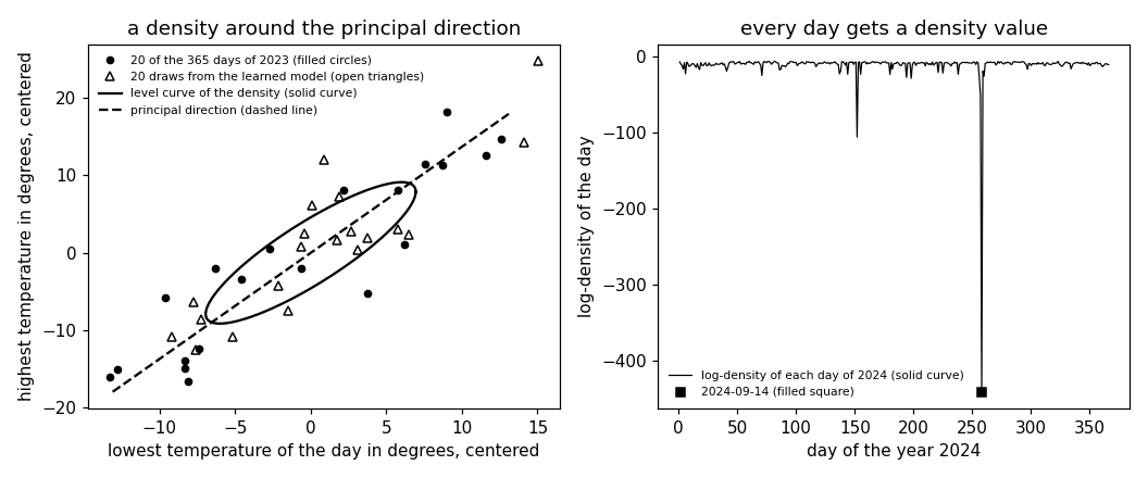
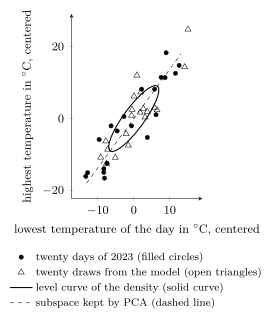
noise produces a new day. Fig. 1
draws the probability distribution \(\eqref{equ_ppca_marginal_dict}\) learned
from the days at Krems taken with two features, the
lowest and the highest temperature of the day, as a level curve
one standard deviation out from the mean vector. For a
code of one number, the subspace that PCA keeps is
a straight line, and the probability distribution fills out an ellipse
around it.
pythondemos/ppca.py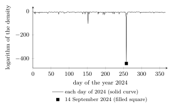
pythondemos/ppca.py
B-emThe expectation–maximization (EM) algorithm reaches the same estimate without an eigenvalue decomposition (EVD) of $\widehat{{\mathbf C}}$, which is the cheaper route when $d$ is large and few directions are wanted (Bishop, 2006, Sect. 12.2.2). Collecting the model parameters ${\mathbf W}$ and $\sigma^{2}$ in ${\mathbf w}$, one iteration is a fixed-point iteration \[{\mathbf w}^{(t+1)} = T \big( {\mathbf w}^{(t)} \big) \text{,}\] whose operator $T$ re-estimates ${\mathbf W}$ from $\widehat{{\mathbf C}}$ and the posterior distribution of the codes, then sets $\sigma^{2}$ to the variance the new ${\mathbf W}$ leaves unexplained (Tipping and Bishop, 1999, Appendix B, Eqs. (29) and (30)). No iteration decreases the likelihood function, and the fixed points of $T$ are the stationary points of that likelihood function. The closed-form estimate is the one among them at which the likelihood function attains its maximum; the stationary points built from eigenvectors other than the leading $d'$ are saddle points (Tipping and Bishop, 1999, Appendix A.3).
B-ermIn the vocabulary of empirical risk minimization (ERM), probabilistic PCA changes two of the three parts of PCA and keeps the third. The hypothesis space gains one number. PCA searches over the products of an encoder and a decoder, which are the matrices of rank at most $d'$. Probabilistic PCA searches over the multivariate normal distributions \(\eqref{equ_ppca_marginal_dict}\), whose covariance matrices are such a matrix plus $\sigma^{2} \mathbf{I}$. The columns of ${\mathbf W}$ need not be orthonormal: those of $\widehat{{\mathbf W}}$ have squared lengths $\lambda_{j} - \widehat{\sigma}^{2}$, for $j = 1, \ldots, d'$, so they fix the variance along each retained direction and not only the subspace. The loss function is the negative logarithm of the pdf of the probability distribution $\mathbb{P}$ \(\eqref{equ_ppca_marginal_dict}\), in place of the squared error loss of PCA, \[L\left({\mathbf x},\mathbb{P} \right) = - \ln \mathcal{N}\left({\mathbf x} \,;\, {\boldsymbol \mu}, {\mathbf C}\right) \text{,}\] so minimizing the empirical risk is maximum likelihood. The third part is unchanged: the EVD of $\widehat{{\mathbf C}}$ that solves PCA delivers this minimum in closed form as well, and the EM algorithm is the route that avoids it. The two loss functions meet as the noise variance tends to zero: $2 \sigma^{2}$ times the empirical risk tends to the minimum reconstruction error $\sum_{j = d' + 1}^{d} \lambda_{j}$ of PCA (Tipping and Bishop, 1999, Appendix A.2, Eq. (17)). That sum is $1.636$ for the eight standardized measurements of the $365$ days of 2023 with $d' = 3$. Multiplied by $2 \sigma^{2}$, the empirical risk reaches $0.979$ of it at $\sigma^{2} = 10^{-2}$, $0.998$ at $10^{-4}$, and $1.000$ at $10^{-6}$.
B-limitA data point is placed in the subspace through the posterior distribution of its code. The posterior mean of the code is \begin{equation} \label{equ_ppca_postmean_dict} \mathbb{E} \big\{ {\mathbf z} \mid {\mathbf x} \big\} = \big( \widehat{{\mathbf W}}^{\top} \widehat{{\mathbf W}} + \widehat{\sigma}^{2} \mathbf{I} \big)^{-1} \widehat{{\mathbf W}}^{\top} \big( {\mathbf x} - \widehat{\boldsymbol \mu} \big) \text{,} \end{equation} whose $j$-th entry, for the closed-form estimate, is the $j$-th PCA coordinate $\langle \mathbf{u}^{(j)}, {\mathbf x} - \widehat{\boldsymbol \mu} \rangle$ multiplied by $\sqrt{\lambda_{j} - \widehat{\sigma}^{2}} \big/ \lambda_{j}$, a factor below one, for $j = 1, \ldots, d'$. The code is therefore pulled toward the origin, by the factors $0.50$, $0.71$, and $0.78$ for the three retained directions at Krems. As $\widehat{\sigma}^{2}$ tends to zero each factor tends to one, and the posterior mean \(\eqref{equ_ppca_postmean_dict}\) becomes the orthogonal projection of the feature vector on the subspace spanned by the first $d'$ eigenvectors, which is what PCA computes (Bishop, 2006, Sect. 12.2.1, Eq. (12.50); Tipping and Bishop, 1999, Sect. 3.4, Eq. (9)). At that limit the covariance matrix ${\mathbf C}$ is singular and the pdf ceases to exist, so the limit that recovers PCA is the one that gives up the probability distribution.
B-missingA probability distribution over the feature space also handles missing data. Conditioned on the entries of a feature vector that were recorded, the probability distribution \(\eqref{equ_ppca_marginal_dict}\) is again Gaussian in the entries that were not, and its expectation is the filled-in value. Deleting the highest temperature of each of the $366$ days of 2024 and filling it in this way, from the model parameters learned on 2023, leaves a mean squared error (MSE) whose square root is $2.28$ degrees, against $9.21$ degrees for filling in the 2023 average instead. The projection that PCA applies needs every entry of the feature vector and offers no such rule, while the same conditional reading lets the model parameters be learned from feature vectors with entries missing (Tipping and Bishop, 1999, Sect. 4.1).
B-costsThe model makes two assumptions, and the days at Krems show what each one costs. The noise is isotropic, so every direction orthogonal to the retained subspace is given the same variance $\widehat{\sigma}^{2} = 0.33$ for the eight standardized measurements with $d' = 3$. The mean air temperature of a day is the average of its lowest and its highest to within $0.05$ degrees on every day of 2023. The sample standard deviation of the days along the last eigenvector of $\widehat{{\mathbf C}}$ is therefore $0.0027$, where the model expects $\widehat{\sigma} = 0.57$. The isotropic noise also makes the learned subspace depend on the units of the measurements: multiplying the precipitation reading by ten turns it by $51$ degrees, the largest angle between the subspace before and after the rescaling. That is why the eight measurements are standardized before the model parameters are learned. Factor analysis differs from probabilistic PCA only in giving the noise a covariance matrix that is a diagonal matrix, one variance per measurement, and a rescaling of one measurement leaves it unchanged (Bishop, 2006, Sect. 12.2.4; Tipping and Bishop, 1999, Sects. 2.1 and 3.3). With its model parameters learned from the same $365$ days of 2023, it raises the median logarithm of the pdf over the $366$ days of 2024 from $-8.5$ to $-3.2$, and what it gives up is the closed form (Tipping and Bishop, 1999, Sect. 2.1).
The second assumption is the Gaussian shape of the pdf \(\eqref{equ_ppca_marginal_dict}\), on which the ranking of days by density value depends. If the days of 2024 were realizations of i.i.d. random vectors with the learned multivariate normal distribution, the quadratic form in the exponent of that pdf would be a realization of a chi-squared random variable (RV) with eight degrees of freedom. Its $99$th percentile is $20.1$, which $3.7$ of the $366$ days would exceed on average. Twenty-six do, as do $16$ of the $365$ days of 2023 the model parameters were learned from. For 14 September 2024, the quadratic form is $870.6$, which the same chi-squared RV exceeds with probability $1.2 \cdot 10^{-182}$, and that day occurred. The density value therefore ranks days, and it does not say how often a day of that kind occurs. Where one multivariate normal distribution is too simple, the standard extension is a mixture of probabilistic PCA models, a Gaussian mixture model (GMM) whose component covariance matrices are each of the form ${\mathbf W} {\mathbf W}^{\top} + \sigma^{2} \mathbf{I}$ (Tipping and Bishop, 1999, Sect. 4.2). What the two assumptions buy in return is a probability distribution over the whole feature space in closed form: it gives a density value to a day outside the training set and a filled-in value to a feature that was not recorded.
See also: principal component analysis, robust principal component analysis, sparse principal component analysis, dimensionality reduction, empirical risk minimization, probabilistic model, multivariate normal distribution, maximum likelihood, expectation–maximization, latent variable, generative model, sample covariance matrix, missing data, anomaly detection, Gaussian mixture model.
@misc{dictml_ppca,
  author = {Jung, Alexander},
  editor = {Olioumtsevits, Konstantina and Schnoor, Ekkehard},
  title = {probabilistic principal component analysis (probabilistic PCA)},
  howpublished = {Dictionary of Applied Machine Learning (course edition)},
  year = {2026},
  doi = {10.5281/zenodo.21569296},
  note = {ISBN 978-952-64-3013-3, CC BY 4.0, retrieved 2026-11-20},
  url = {https://dictionaryofml.org/terms/ppca.html}
}