encoder.py, which recomputes what the entry states: the script block by block · open in ColabDictionary of Applied Machine Learning: 147 machine-learning terms, each with a definition, a figure, citations and a Python demo · All terms · Demos · Start here
Updated on 2026-11-20
Readiness 90/100
See also decoder autoencoder feature learning feature transformation dimensionality reduction principal component analysis linear discriminant analysis empirical risk minimization squared error loss
An encoder is a map that sends the raw feature vector of a data point to a shorter vector, a code of $d'$ numbers with $d'$ below the number $d$ of raw features. Its counterpart is the decoder, which maps a code back to a vector of the original length, and the two are judged together: the decoder applied to the code of a data point should return approximately the feature vector the encoder started from. The average loss that remains, the reconstruction error, is what training minimizes. Principal component analysis (PCA) uses a linear map as the encoder, a matrix whose rows are the eigenvectors of the sample covariance matrix belonging to its largest eigenvalues. An autoencoder learns the encoder jointly with the decoder, so it can be a deep net rather than a linear map. A large language model (LLM) begins with the token-to-vector encoder, which carries every token of a vocabulary to one row of an embedding matrix. The code length decides what the decoder can rebuild, and the code kept in place of the raw feature vectors is what makes an encoder a feature transformation for a later learning task. What a shorter code drops is beyond every decoder, so a code learned to reconstruct well need not serve that learning task well.
encoder.py, which recomputes what the entry states: the script block by block · open in ColabThe weather station at Krems an der Donau (Austria) records eight numbers for each day: the lowest, the highest, and the mean air temperature, the precipitation, the sunshine duration, the humidity, the air pressure, and the wind speed. Two numbers computed from the eight are enough to tell a day in January from a day in July, and a second map rebuilds the eight from the two with a small error. The map that delivers the two numbers is an encoder. It sends the raw feature vector ${\mathbf x} \in \mathbb{R}^{d}$ of a data point to a shorter vector ${\mathbf z} \in \mathbb{R}^{d'}$, its code, \[{\mathbf \Phi}: \mathbb{R}^{d} \rightarrow \mathbb{R}^{d'}: {\mathbf x} \mapsto {\mathbf z} := {\mathbf \Phi}({\mathbf x}) \text{,}\] with a code length $d'$ below the number $d$ of raw features. Its counterpart is the decoder ${\mathbf \Phi}^{*}: \mathbb{R}^{d'} \rightarrow \mathbb{R}^{d}$, which maps a code back to a vector with $d$ entries (Goodfellow et al., 2016, Ch. 14).
B-encoderEncoders differ in the hypothesis space they are picked from. Principal component analysis (PCA) picks a linear map: the encoder is a matrix ${\mathbf W} \in \mathbb{R}^{d' \times d}$ with ${\mathbf z} = {\mathbf W} {\mathbf x}$, whose rows are the eigenvectors of the sample covariance matrix of the feature vectors belonging to its $d'$ largest eigenvalues, and the decoder is the transpose ${\mathbf W}^{\top}$ (Bishop, 2006, Sect. 12.1.2; Hotelling, 1933). An autoencoder picks the encoder from a hypothesis space of deep nets and learns it jointly with the decoder, so that neither map need be linear (Goodfellow et al., 2016, Sect. 14.1). A large language model (LLM) begins with the token-to-vector step, an encoder on text. Every token of a vocabulary $\mathcal{V}$ carries one row of an embedding matrix $\mathbf{E} \in \mathbb{R}^{|\mathcal{V}| \times d'}$. Picking the row of the token with index $v$ is the linear map ${\mathbf z} = \mathbf{E}^{\top} {\mathbf e}^{(v)}$ applied to the one-hot vector ${\mathbf e}^{(v)} \in \mathbb{R}^{|\mathcal{V}|}$ of that token (Vaswani et al., 2017, Sect. 3.4).
What makes a code useful is that the decoder can rebuild the data point from it. The reconstruction error of an encoder on a dataset $\mathcal{D} = \{{\mathbf x}^{(1)}, \ldots, {\mathbf x}^{(m)}\}$ of sample size $m$ is the average loss between a feature vector and what the decoder returns for its code, \begin{equation} \label{equ_encoder_reconstruction_dict} \frac{1}{m} \sum_{r=1}^{m} L\left({\mathbf x}^{(r)},{\mathbf \Phi}^{*} \big( {\mathbf \Phi} \big( {\mathbf x}^{(r)} \big) \big) \right) \text{.} \end{equation} A common loss function is the squared error loss $\left\lVert {\mathbf x} - {\mathbf \Phi}^{*}({\mathbf \Phi}({\mathbf x})) \right\rVert_{2}^{2}$, and minimizing the reconstruction error \(\eqref{equ_encoder_reconstruction_dict}\) over a hypothesis space of encoders and a second one of decoders is empirical risk minimization (ERM). No labels enter it: what the decoder has to reproduce is the data point itself, so the training of an encoder is a form of self-supervised learning.
B-lengthEach of the eight measurements of a day at Krems is scaled to zero
sample mean and unit sample variance, so that they carry
comparable weight. Over the $366$ days of $2024$, the PCA encoder with
$d' = 2$ then leaves a reconstruction error of $2.91$ out
of the total variance $8.00$, and the eight reconstructed
measurements of 1 January 2024 differ from the scaled originals by
at most $0.80$.
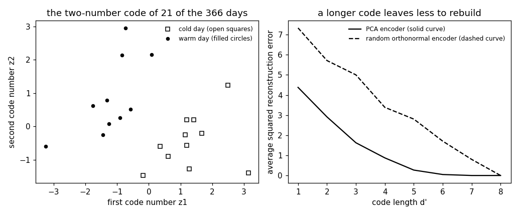
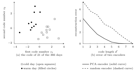
Fig. 1(a) places $21$ of the days at their two
code numbers, split at the median of the maximum
temperature, and Fig. 1(b) compares the
reconstruction error of this encoder with what a random encoder
with orthonormal rows leaves as the code grows.
pythondemos/encoder.py
B-dropsThe code of two numbers leaves a reconstruction error of $2.91$, and that loss is not spread evenly over the eight measurements. Of the unit sample variance of each measurement, the code keeps $96$ percent of the mean temperature and $3$ percent of the wind speed. What the dropped eigenvectors carried is beyond every decoder, not only the transpose ${\mathbf W}^{\top}$. Of the $80$ pairs of days whose codes lie closer than $0.1$ together, 14 February and 22 November 2024 differ most in wind speed, $1.0$ against $4.5$ meters per second, and the decoder returns $1.76$ meters per second for both. Whether the loss matters is decided by the later learning task and not by the reconstruction error alone. A day counts as windy when its mean wind speed lies above the median of the $366$ values, which holds for $130$ of them. A linear classifier learned by least squares has an accuracy of $98$ percent from all eight scaled measurements and $66$ percent from the two code numbers, against the $64$ percent reached by calling every day calm. One new feature chosen from the labels instead of from the sample covariance matrix, the linear discriminant analysis (LDA) direction, reaches $98$ percent as well. A code learned to reconstruct well is therefore not a code learned to predict well, which is the difference LDA draws against PCA. An encoder is also fixed once learned, and the dataset it was learned from decides how well it codes a later day. The PCA encoder of the $183$ days of January to March and of October to December leaves $1.93$ on those days and $10.87$ on the other $183$, against $2.48$ for the encoder of the whole year. What the code buys is its shortness: fewer numbers per data point to store and to hand to a later learning task, and at $d' = 2$ a plot of the dataset on two axes.
See also: decoder, autoencoder, variational autoencoder, feature learning, feature transformation, dimensionality reduction, principal component analysis, linear discriminant analysis, embedding, token, latent variable, empirical risk minimization, squared error loss.
@misc{dictml_encoder,
  author = {Jung, Alexander},
  editor = {Olioumtsevits, Konstantina and Schnoor, Ekkehard},
  title = {encoder},
  howpublished = {Dictionary of Applied Machine Learning (course edition)},
  year = {2026},
  doi = {10.5281/zenodo.21569296},
  note = {ISBN 978-952-64-3013-3, CC BY 4.0, retrieved 2026-11-20},
  url = {https://dictionaryofml.org/terms/encoder.html}
}