decoder.py, which recomputes what the entry states: the script block by block · open in ColabDictionary of Applied Machine Learning: 147 machine-learning terms, each with a definition, a figure, citations and a Python demo · All terms · Demos · Start here
Updated on 2026-11-20
Readiness 95/100
See also encoder autoencoder principal component analysis feature learning dimensionality reduction feature transformation empirical risk minimization squared error loss eigenvector large language model
A decoder is a map that turns the code of a data point, the short vector an encoder computes from it, back into the space the data point itself lives in. The encoder and the decoder are learned together by empirical risk minimization (ERM), with a loss function that measures the reconstruction error between a data point and what the decoder returns for its code. In principal component analysis (PCA) both maps are linear and the decoder is the transpose of the encoder, so the reconstruction is the orthogonal projection of the feature vector onto the subspace spanned by the retained eigenvectors, and the average squared reconstruction error is the sum of the discarded eigenvalues. An autoencoder replaces both linear maps by artificial neural networks (ANNs), and its decoder is often discarded once the code is wanted for a later learning task. A decoder may return a probability distribution instead of a point: the decoder of a variational autoencoder (VAE) is a conditional probability distribution over feature vectors given a latent variable. The output step of a large language model (LLM) is a decoder as well, turning a vector into a probability distribution over the vocabulary, which is what lets text be generated one token at a time.
decoder.py, which recomputes what the entry states: the script block by block · open in ColabThe weather station at Krems an der Donau (Austria) records the lowest and the highest air temperature of each day, so a day is a point of the plane with these two features as its coordinates. Storing one number per day instead of two is possible, but that number is of no use unless some map turns it back into a pair of temperatures. A decoder is such a map.
B-projectionA decoder is a map ${\mathbf \Phi}^{*}: \mathcal{X}'
\rightarrow \mathcal{X}$ from a space $\mathcal{X}'$ of codes
back to the feature space $\mathcal{X}$ that holds the
feature vector ${\mathbf x}$ of a data point. Its
counterpart is the encoder ${\mathbf \Phi}: \mathcal{X}
\rightarrow \mathcal{X}'$, which computes the code ${\mathbf z} =
{\mathbf \Phi}({\mathbf x})$, a vector of $d'$
numbers against the $d$ numbers of the feature vector,
with $d' < d$. The two maps form an
autoencoder, and they are learned together by empirical risk minimization (ERM) with
a loss function that measures the reconstruction error
${\mathbf x} -
{\mathbf \Phi}^{*}({\mathbf \Phi}({\mathbf x}))$
(Goodfellow et al., 2016, Sect. 14.1). No label enters
this learning task: what the decoder has to reproduce is the
data point itself. What the decoder returns need not be a
point of $\mathcal{X}$: it may be a probability distribution, over
$\mathcal{X}$ or over a vocabulary of tokens.
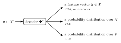
Fig. 1 shows the three shapes the
decoder takes in principal component analysis (PCA), in a variational autoencoder (VAE), and in a large language model (LLM).
B-eigenvaluesThe eigenvalues of $\widehat{\mathbf{Q}}$, in decreasing order
$\lambda_{1} \geq \cdots \geq \lambda_{d} \geq 0$, state
what every code length costs. For a dataset $\mathcal{D} =
\{{\mathbf x}^{(1)}, \ldots, {\mathbf x}^{(m)}\}$ of
feature vectors with sample mean zero, the average squared
reconstruction error is the sum of the eigenvalues the code
drops (Bishop, 2006, Sect. 12.1.2, Eq. (12.18)),
\begin{equation}
\label{equ_decoder_eigenvalues_dict}
\frac{1}{m} \sum_{r=1}^{m}
\left\lVert {\mathbf x}^{(r)} - {\mathbf W}^{\top} {\mathbf W}
{\mathbf x}^{(r)} \right\rVert_{2}^{2} =
\sum_{j=d'+1}^{d}
\lambda_{j} \text{.}
\end{equation}
The identity \(\eqref{equ_decoder_eigenvalues_dict}\) holds at every
code length $d' = 1, \ldots, d$. The archive at
Krems holds eight measurements per day: the lowest, highest and
mean air temperature, the precipitation, the sunshine duration, the
humidity, the air pressure, and the wind speed. Each of the eight
is scaled to unit sample variance, because they are measured
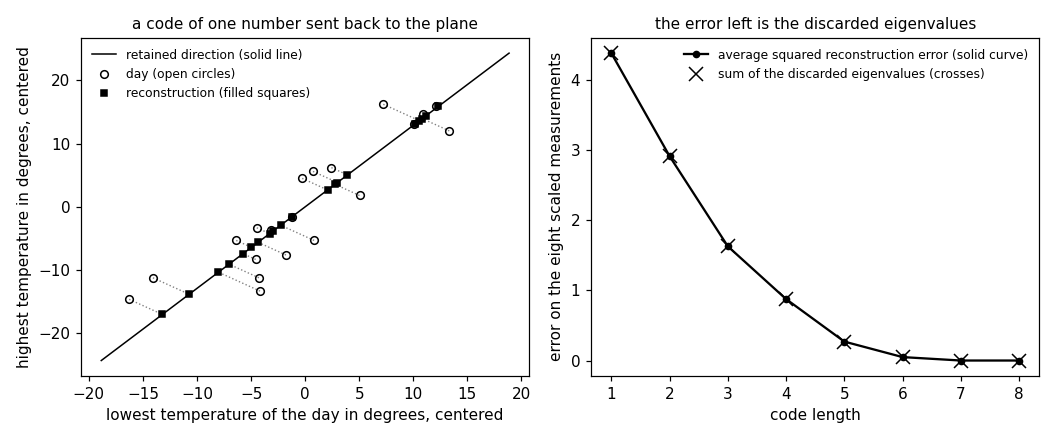
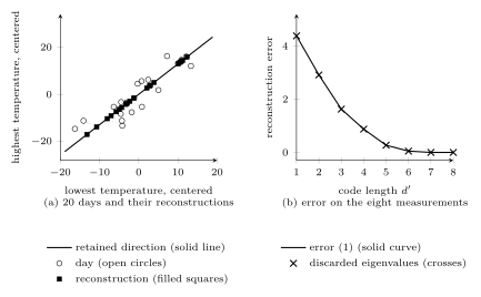
in different units. A code of two numbers then leaves $2.91$ of the
total $8$, so the decoder recovers $64$ percent of the total
sample variance. Fig. 2 draws the
decoder of a code of one number for the two temperatures, and both
sides of the identity \(\eqref{equ_decoder_eigenvalues_dict}\) at
every code length.
pythondemos/decoder.py
B-gaussA decoder need not return a point. The decoder of a VAE is a conditional probability distribution $p_{{\mathbf w}}({\mathbf x} \mid {\mathbf z})$ over feature vectors given a latent variable ${\mathbf z}$, with model parameters ${\mathbf w}$: given a code it returns a probability distribution over the feature vectors that could have produced it (Kingma and Welling, 2014, Sect. 2.1). Drawing ${\mathbf z}$ from a fixed probability distribution and then a feature vector from the decoder makes the pair a generative model. The two readings meet where that conditional probability distribution is Gaussian with mean ${\mathbf R} {\mathbf z}$, for a matrix ${\mathbf R} \in \mathbb{R}^{d \times d'}$, and a spread that does not depend on ${\mathbf z}$. Its log-likelihood function is then a decreasing affine function of the average squared reconstruction error, so the matrix ${\mathbf R}$ that maximizes the one minimizes the other.
The step that turns a vector into text is a decoder too. An LLM computes a vector ${\mathbf z} \in \mathbb{R}^{d}$ from the tokens read so far. The decoder maps it to a probability distribution over the vocabulary $\mathcal{V}$ by a linear map followed by the softmax function (Vaswani et al., 2017, Sect. 3.4). The rows of that linear map are ${\mathbf a}^{(1)}, \ldots, {\mathbf a}^{(|\mathcal{V}|)} \in \mathbb{R}^{d}$, and the decoder returns \begin{equation} \label{equ_decoder_vocabulary_dict} \big( {\mathbf \Phi}^{*}({\mathbf z}) \big)_{v} = \frac{\exp \big( \langle {\mathbf a}^{(v)}, {\mathbf z} \rangle \big)} {\sum_{v'=1}^{|\mathcal{V}|} \exp \big( \langle {\mathbf a}^{(v')}, {\mathbf z} \rangle \big)} \quad \text{for } v = 1, \ldots, |\mathcal{V}| \text{.} \end{equation} Every value the quotient \(\eqref{equ_decoder_vocabulary_dict}\) assigns is nonnegative, and the values sum to one over $v = 1, \ldots, |\mathcal{V}|$, so the decoder returns a point of the probability simplex $\Delta^{|\mathcal{V}|-1}$. Drawing one token from that probability distribution, appending it to the tokens read so far, and repeating is how text is generated one token at a time (Vaswani et al., 2017, Sect. 3): without the decoder, the vector ${\mathbf z}$ names no token at all.
B-vocabularyA vocabulary of eight tokens is already enough to check the decoder \(\eqref{equ_decoder_vocabulary_dict}\) numerically. Cutting the highest temperature of each day at Krems into eight bins of about $45$ days each, and choosing the rows ${\mathbf a}^{(v)}$ by maximum likelihood, reproduces the observed frequencies of the next token to within $0.0014$. A sequence of $20{,}001$ tokens generated one at a time then matches the observed shares of the eight tokens to within $0.009$.
B-limitsThe reconstructions of a linear decoder lie in a subspace of dimension $d'$, whatever the dataset looks like. The identity \(\eqref{equ_decoder_eigenvalues_dict}\) says what that costs on average, and nothing about where the reconstructions land. Read back in the recorded units, the reconstruction of a day from a code of two numbers gives $128$ of the $366$ days a negative precipitation, down to $-7.3$ millimeters, and $17$ days a negative sunshine duration. No day of the record takes a negative value in either measurement. A linear decoder learned with the squared error loss recovers the subspace PCA finds, so only a nonlinear decoder places a reconstruction off a subspace (Goodfellow et al., 2016, Sect. 14.1), which is why the decoder of an autoencoder is an ANN and not a matrix.
B-plotWhat the linear decoder buys is a closed form: its eigenvectors come from the sample covariance matrix with no training run, and its eigenvalues state the error of every code length in advance. Curving the reconstruction set does not always lower the error: with the same code of one number, the average of the days in each of eight bins leaves $5.10$ on days it was not learned from, against the $5.07$ of the linear decoder.
A decoder that returns a probability distribution rather than a point buys a probability for every reconstruction and the ability to generate, since a feature vector or a token can be drawn from what the decoder returns. The price is a probabilistic model that has to be learned and can be wrong, and a support fixed in advance. The Gaussian decoder above commits to a spread that does not depend on the code. The vocabulary of eight tokens resolves the maximum daytime temperature of a day only to its bin: $1.4$ degrees in root mean square, and $10.3$ degrees for the coldest token, which holds every day at or below $6.7$ degrees. No sequence of these eight tokens tells two days of one bin apart.
See also: encoder, autoencoder, denoising autoencoder, variational autoencoder, latent variable, conditional probability distribution, probabilistic model, principal component analysis, feature learning, dimensionality reduction, feature transformation, empirical risk minimization, squared error loss, orthogonal projection, subspace, eigenvector, generative model, softmax function, probability simplex, vocabulary, large language model.
@misc{dictml_decoder,
  author = {Jung, Alexander},
  editor = {Olioumtsevits, Konstantina and Schnoor, Ekkehard},
  title = {decoder},
  howpublished = {Dictionary of Applied Machine Learning (course edition)},
  year = {2026},
  doi = {10.5281/zenodo.21569296},
  note = {ISBN 978-952-64-3013-3, CC BY 4.0, retrieved 2026-11-20},
  url = {https://dictionaryofml.org/terms/decoder.html}
}