B-plot writes when the script runsDictionary of Applied Machine Learning · probabilistic principal component analysis (probabilistic PCA)
Updated on 2026-11-20
Numerical companion to the entry probabilistic principal component analysis (probabilistic PCA): it recomputes what the entry states and prints one line per check
Numerical companion to the glossary entry 'ppca' (probabilistic principal component analysis). The GeoSphere Austria weather station Krems (station id 3805) records eight measurements per day: lowest, highest and mean air temperature, precipitation, sunshine duration, relative humidity, air pressure and wind speed. A value of -1 for precipitation marks a trace of rain too small to record and is set to 0.
Run it without installing anything:uv run https://dictionaryofml.org/terms/ppca.py
uv downloads this script and the pinned NumPy and Matplotlib it needs, then runs it; the script fetches any input file it uses. To keep the output files, download ppca.py into a folder and run uv run ppca.py there. With NumPy and Matplotlib already installed, python3 ppca.py, from any directory — it writes its output files into the current directory. Fixed seeds, so the printed numbers reproduce exactly. Download ppca.py · Notebook · Open in Colab
Before running a downloaded copy, scan it: uvx bandit -q -t B102,B307,B602,B605 ppca.py (B102,B307,B602,B605 are the exec, eval and shell checks of bandit) reports nothing: the script runs no shell command and evaluates no generated code.
One cell per block of the script: the code, and what that code printed when it last ran here
"""Probabilistic PCA on the days at Krems an der Donau: a latent Gaussian
code, a matrix and isotropic Gaussian noise give a density over the
measurements of a day, whose maximum likelihood estimate is read off the
eigenvalues of the sample covariance matrix.

Purpose
-------
Numerical companion to the glossary entry 'ppca' (probabilistic principal
component analysis).  The GeoSphere Austria weather station Krems
(station id 3805) records eight measurements per day: lowest, highest and
mean air temperature, precipitation, sunshine duration, relative
humidity, air pressure and wind speed.  A value of -1 for precipitation
marks a trace of rain too small to record and is set to 0.

Probabilistic PCA models the feature vector of a day as x = W z + mu + e,
with a latent code z drawn from a zero-mean unit-covariance Gaussian, a
d x d' matrix W, and isotropic Gaussian noise e of variance sigma^2.  The
feature vector is then Gaussian with mean mu and covariance
C = W W^T + sigma^2 I, so every day gets a probability density value.

The demo checks the entry's claims: (1) the covariance C of the model
has the retained eigenvalues of the sample covariance matrix along the
principal directions and sigma^2 in every direction orthogonal to them;
(2) the maximum likelihood estimate has a closed form in those
eigenvalues, with sigma^2 the average of the discarded ones, and it beats
random parameters and a grid over sigma^2; (3) the EM algorithm is a
fixed-point iteration whose fixed point is that closed form; (4) the loss
-log p is the one PCA minimizes in the limit of vanishing noise, since
2 sigma^2 times its average over the training set tends to the minimum
reconstruction error of PCA; (5) the posterior mean of the latent code is
a shrunk version of the PCA coordinates and becomes the orthogonal
projection as sigma^2 tends to zero; (6) the density scores a day that did
not belong to the training set, and the least probable day of 2024 is the
day of the September flood; (7) the same density fills in a missing
reading by a conditional mean; and (8) both assumptions of the model fail
on this
record: the days nearly satisfy a linear relation that the single noise
variance cannot hold, the learned subspace depends on the units of the
measurements, factor analysis with one variance per measurement scores
the held-out days higher, and far more days of 2024 fall in the tail of
the density than a Gaussian allows.

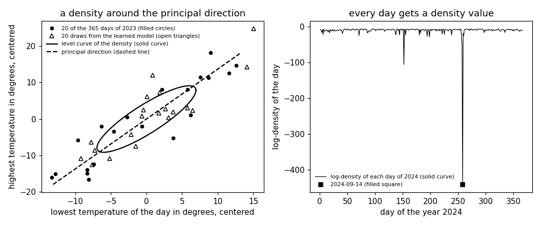
Two views of the same data, as in the 'pca' demo.  The picture uses the
two temperatures in degrees Celsius, centered but not rescaled, so the
density can be drawn in the units of the measurement.  The numbers quoted
for the eight measurements use all of them, each scaled to zero sample
mean and unit variance on the 2023 days because temperatures,
precipitation and pressure carry different units.

Self-contained (numpy and matplotlib only), fixed seeds; the GeoSphere
download falls back to the committed CSV.

Blocks
------
[B-data]    The eight measurements for the 365 days of 2023 and the 366
            days of 2024; the two temperatures centered for the picture
            and all eight scaled for the numbers.
[B-model]   The model covariance C = W W^T + sigma^2 I: its eigenvalues,
            and the sample covariance matrix of a large number of draws.
[B-mle]     The closed-form maximum likelihood estimate: sigma^2 is the
            average of the discarded eigenvalues, and the estimate beats
            2000 random parameter sets and a grid over sigma^2.
[B-em]      EM as a fixed-point iteration: it reaches the log-likelihood
            of the closed form, and the closed form is a fixed point of
            the EM map.
[B-erm]     Maximum likelihood as empirical risk minimization: the loss
            is -log p, and 2 sigma^2 times its average over the training
            set tends to the minimum reconstruction error of PCA as the
            noise variance tends to zero.
[B-limit]   The posterior mean of the latent code shrinks the PCA
            coordinates by a known factor and becomes the orthogonal
            projection as sigma^2 tends to zero.
[B-density] A density for every day: the log-density of the 366 days of
            2024 under the model learned on the 365 days of 2023, and the
            least probable day of 2024.
[B-missing] The conditional mean under the same density fills in a
            deleted highest-temperature reading.
[B-costs]   Where the two assumptions fail: the isotropic noise against
            the near-exact linear relation among the three temperatures
            and against a rescaled measurement, factor analysis as the
            alternative, and the Gaussian tail against the number of
            days of 2024 that fall into it.
[B-plot]    Preview: the days of 2023 in the two temperatures with draws
            from the model and a level curve of its density, and the
            log-density of each day of 2024 over the year.

Outputs
-------
ppca_weather.csv     : date and the eight measurements, 2023 and 2024
ppca_points_plot.csv : x1, x2 -- the centered temperatures of the 20 of
                       the 365 days of 2023 the figure draws (every 19th)
ppca_draws_plot.csv  : x1, x2 -- 20 draws from the learned model
ppca_ellipse.csv     : x1, x2 -- the level curve of the density one
                       standard deviation out
ppca_axis.csv        : x1, x2 -- the principal direction as a segment
ppca_logdens.csv     : day of the year and the log-density of that day of
                       2024 under the learned model
ppca.png             : matplotlib preview (checking only)
"""

# /// script
# requires-python = ">=3.10"
# dependencies = ["matplotlib==3.10.7", "numpy==2.3.4"]
# ///

import json
import math
import urllib.request
from pathlib import Path

import numpy as np
import matplotlib

matplotlib.use("Agg")
import matplotlib.pyplot as plt

OUT_DIR = Path(__file__).parent

report = []


def check(name, ok):
    report.append((name, bool(ok)))
    print(f"  [{'ok' if ok else 'FAIL'}] {name}")
The eight measurements for the 365 days of 2023 and the 366 days of 2024; the two temperatures centered for the picture and all eight scaled for the numbers.
print("[B-data] the eight measurements at Krems for 2023 and 2024")
PARAMS = ["tlmin", "tlmax", "tl_mittel", "rr", "so_h", "rf_mittel",
          "p_mittel", "vv_mittel"]
URL = ("https://dataset.api.hub.geosphere.at/v1/station/historical/"
       f"klima-v2-1d?parameters={','.join(PARAMS)}&station_ids=3805"
       "&start=2023-01-01&end=2024-12-31")
CSV = OUT_DIR / "ppca_weather.csv"
try:
    with urllib.request.urlopen(URL, timeout=180) as resp:
        payload = json.load(resp)
    params = payload["features"][0]["properties"]["parameters"]
    stamps = [t[:10] for t in payload["timestamps"]]
    M = np.stack([np.array(params[p]["data"], dtype=float) for p in PARAMS], 1)
    M[:, 3] = np.maximum(M[:, 3], 0.0)         # -1 marks a trace of rain
    with open(CSV, "w") as fh:
        fh.write("date," + ",".join(PARAMS) + "\n")
        for day, row in zip(stamps, M):
            fh.write(day + "," + ",".join(f"{v:g}" for v in row) + "\n")
    print(f"    downloaded {len(stamps)} days")
except OSError as err:
    print(f"    download failed ({err}); reading the committed CSV")
    rows = CSV.read_text().strip().splitlines()[1:]
    stamps = [r.split(",")[0] for r in rows]
    M = np.array([[float(v) for v in r.split(",")[1:]] for r in rows])

is23 = np.array([s.startswith("2023") for s in stamps])
check("[B-data] 365 days of 2023 and 366 days of 2024, eight measurements "
      "each", M.shape == (731, 8) and is23.sum() == 365)
check("[B-data] no measurement is missing", not np.isnan(M).any())
check("[B-data] the record matches the archive (1 February 2024: lowest "
      "-3.8, highest 10.4 degrees)",
      stamps[396] == "2024-02-01" and np.allclose(M[396, :2], [-3.8, 10.4]))

T = M[is23, :2] - M[is23, :2].mean(axis=0)     # two temperatures, centered
mu8, sd8 = M[is23].mean(axis=0), M[is23].std(axis=0)
X23 = (M[is23] - mu8) / sd8                    # all eight, scaled on 2023
X24 = (M[~is23] - mu8) / sd8
m23, m24, d = len(X23), len(X24), M.shape[1]
check("[B-data] the two temperatures of the picture are centered",
      np.allclose(T.mean(axis=0), 0))


def principal(A):
    """Eigenvalues and eigenvectors of the sample covariance matrix of the
    centered rows of A, in decreasing order of eigenvalue."""
    B = A - A.mean(axis=0)
    vals, vecs = np.linalg.eigh(B.T @ B / len(B))
    order = np.argsort(vals)[::-1]
    return vals[order], vecs[:, order]


def ppca_mle(A, dp):
    """Closed-form maximum likelihood estimate of the model parameters for
    a code of dp numbers: the sample mean, W = U (L - sigma^2 I)^(1/2) and
    sigma^2 the average of the discarded eigenvalues."""
    vals, vecs = principal(A)
    sig2 = float(vals[dp:].mean())
    W = vecs[:, :dp] * np.sqrt(np.maximum(vals[:dp] - sig2, 0.0))
    return A.mean(axis=0), W, sig2, vals, vecs


def log_density_cov(A, mean, C):
    """Log of the density of a multivariate normal distribution with the
    given mean vector and covariance matrix at every row of A."""
    _, logdet = np.linalg.slogdet(C)
    B = A - mean
    quad = np.einsum("ij,jk,ik->i", B, np.linalg.inv(C), B)
    return -0.5 * (A.shape[1] * np.log(2 * np.pi) + logdet + quad)


def log_density(A, mean, W, sig2):
    """Log of the density of the model at every row of A."""
    dim = A.shape[1]
    return log_density_cov(A, mean, W @ W.T + sig2 * np.eye(dim))
[B-data] the eight measurements at Krems for 2023 and 2024
    downloaded 731 days
  [ok] [B-data] 365 days of 2023 and 366 days of 2024, eight measurements each
  [ok] [B-data] no measurement is missing
  [ok] [B-data] the record matches the archive (1 February 2024: lowest -3.8, highest 10.4 degrees)
  [ok] [B-data] the two temperatures of the picture are centered
The model covariance C = W W^T + sigma^2 I: its eigenvalues, and the sample covariance matrix of a large number of draws.
print("[B-model] the covariance of the model and the draws it produces")
DCODE = 3
mean8, W8, sig28, lam8, U8 = ppca_mle(X23, DCODE)
C8 = W8 @ W8.T + sig28 * np.eye(d)
cvals, _ = np.linalg.eigh(C8)
cvals = np.sort(cvals)[::-1]
print(f"    eigenvalues of the sample covariance matrix: "
      f"{np.array2string(lam8, precision=3)}")
print(f"    eigenvalues of C for d' = {DCODE}: "
      f"{np.array2string(cvals, precision=3)}")
check(f"[B-model] C keeps the {DCODE} largest eigenvalues of the sample "
      f"covariance matrix exactly", np.allclose(cvals[:DCODE], lam8[:DCODE]))
check(f"[B-model] C replaces the other {d - DCODE} by sigma^2 = "
      f"{sig28:.4f}, their average", np.allclose(cvals[DCODE:], sig28))
check("[B-model] C is the sum of a matrix of rank d' and a multiple of "
      "the identity matrix",
      np.linalg.matrix_rank(W8 @ W8.T, tol=1e-9) == DCODE)
rng = np.random.default_rng(0)
Z = rng.standard_normal((400000, DCODE))
E = np.sqrt(sig28) * rng.standard_normal((400000, d))
draws8 = Z @ W8.T + mean8 + E
Chat = (draws8 - draws8.mean(axis=0)).T @ (draws8 - draws8.mean(axis=0)) / len(draws8)
check(f"[B-model] 400000 draws W z + mu + e have sample covariance matrix "
      f"within {np.abs(Chat - C8).max():.4f} of C",
      np.abs(Chat - C8).max() < 0.02)
[B-model] the covariance of the model and the draws it produces
    eigenvalues of the sample covariance matrix: [3.578e+00 1.576e+00 1.209e+00 7.718e-01 6.370e-01 1.702e-01 5.737e-02
 7.378e-06]
    eigenvalues of C for d' = 3: [3.578 1.576 1.209 0.327 0.327 0.327 0.327 0.327]
  [ok] [B-model] C keeps the 3 largest eigenvalues of the sample covariance matrix exactly
  [ok] [B-model] C replaces the other 5 by sigma^2 = 0.3273, their average
  [ok] [B-model] C is the sum of a matrix of rank d' and a multiple of the identity matrix
  [ok] [B-model] 400000 draws W z + mu + e have sample covariance matrix within 0.0039 of C
The closed-form maximum likelihood estimate: sigma^2 is the average of the discarded eigenvalues, and the estimate beats 2000 random parameter sets and a grid over sigma^2.
print("[B-mle] the closed-form maximum likelihood estimate")
ll_mle = float(log_density(X23, mean8, W8, sig28).sum())
check(f"[B-mle] sigma^2 = {sig28:.4f} is the average of the "
      f"{d - DCODE} discarded eigenvalues", np.isclose(sig28, lam8[DCODE:].mean()))
worse = 0
for _ in range(2000):
    Wr = rng.standard_normal((d, DCODE)) * np.sqrt(lam8[:DCODE]).mean()
    s2r = float(np.exp(rng.uniform(np.log(1e-3), np.log(2.0))))
    if log_density(X23, mean8, Wr, s2r).sum() < ll_mle:
        worse += 1
check(f"[B-mle] the estimate beats all 2000 random parameter sets "
      f"(log-likelihood {ll_mle:.1f})", worse == 2000)
grid = np.exp(np.linspace(np.log(1e-3), np.log(2.0), 400))
best = max(grid, key=lambda s2: log_density(
    X23, mean8, U8[:, :DCODE] * np.sqrt(np.maximum(lam8[:DCODE] - s2, 0.0)),
    s2).sum())
check(f"[B-mle] a grid of 400 values of sigma^2 is best at {best:.4f}, "
      f"next to the closed form {sig28:.4f}", abs(best - sig28) < 0.02)
[B-mle] the closed-form maximum likelihood estimate
  [ok] [B-mle] sigma^2 = 0.3273 is the average of the 5 discarded eigenvalues
  [ok] [B-mle] the estimate beats all 2000 random parameter sets (log-likelihood -3474.5)
  [ok] [B-mle] a grid of 400 values of sigma^2 is best at 0.3274, next to the closed form 0.3273
EM as a fixed-point iteration: it reaches the log-likelihood of the closed form, and the closed form is a fixed point of the EM map.
print("[B-em] EM as a fixed-point iteration on (W, sigma^2)")


def em_step(A, W, sig2):
    """One EM step for the model parameters, the map T of the entry."""
    dim, dp = W.shape
    B = A - A.mean(axis=0)
    S = B.T @ B / len(B)
    Mi = np.linalg.inv(W.T @ W + sig2 * np.eye(dp))
    SW = S @ W
    Wn = SW @ np.linalg.inv(sig2 * np.eye(dp) + Mi @ W.T @ SW)
    sig2n = float(np.trace(S - SW @ Mi @ Wn.T) / dim)
    return Wn, sig2n


W_em = rng.standard_normal((d, DCODE))
s2_em = 1.0
lls = []
for _ in range(4000):
    W_em, s2_em = em_step(X23, W_em, s2_em)
    lls.append(float(log_density(X23, mean8, W_em, s2_em).sum()))
check("[B-em] every EM step increases the log-likelihood",
      np.all(np.diff(lls) > -1e-6))
check(f"[B-em] EM reaches the log-likelihood of the closed form "
      f"({lls[-1]:.3f} against {ll_mle:.3f})", abs(lls[-1] - ll_mle) < 1e-3)
check(f"[B-em] EM recovers sigma^2 = {s2_em:.4f}", abs(s2_em - sig28) < 1e-4)
C_em = W_em @ W_em.T + s2_em * np.eye(d)
check(f"[B-em] the covariance it delivers agrees with C to "
      f"{np.abs(C_em - C8).max():.2e}, so the rotation of W is the only "
      f"part left open", np.abs(C_em - C8).max() < 1e-4)
W_fix, s2_fix = em_step(X23, W8, sig28)
check(f"[B-em] the closed form is a fixed point of T: one more step moves "
      f"it by {max(np.abs(W_fix - W8).max(), abs(s2_fix - sig28)):.2e}",
      np.abs(W_fix - W8).max() < 1e-10 and abs(s2_fix - sig28) < 1e-10)
[B-em] EM as a fixed-point iteration on (W, sigma^2)
  [ok] [B-em] every EM step increases the log-likelihood
  [ok] [B-em] EM reaches the log-likelihood of the closed form (-3474.488 against -3474.488)
  [ok] [B-em] EM recovers sigma^2 = 0.3273
  [ok] [B-em] the covariance it delivers agrees with C to 1.33e-15, so the rotation of W is the only part left open
  [ok] [B-em] the closed form is a fixed point of T: one more step moves it by 2.78e-16
Maximum likelihood as empirical risk minimization: the loss is -log p, and 2 sigma^2 times its average over the training set tends to the minimum reconstruction error of PCA as the noise variance tends to zero.
print("[B-erm] maximum likelihood as ERM, and the loss as sigma^2 vanishes")


def mean_loss(A, mean, W, sig2):
    """The average of the loss -log p over the rows of A, the empirical
    risk of the negative log density loss."""
    return float(-log_density(A, mean, W, sig2).mean())


def profile_loss(sig2, vals, dim, dp):
    """Twice that average written in the eigenvalues of the sample
    covariance matrix, Eq. (17) of Tipping and Bishop (1999)."""
    return (dim * np.log(2 * np.pi) + float(np.log(vals[:dp]).sum())
            + float(vals[dp:].sum()) / sig2
            + (dim - dp) * np.log(sig2) + dp)


err_pca = float(lam8[DCODE:].sum())
proj = U8[:, :DCODE] @ U8[:, :DCODE].T
cen = X23 - mean8
dist2 = ((cen - cen @ proj) ** 2).sum(axis=1)
colnorm = np.linalg.norm(W8, axis=0)
check(f"[B-erm] the columns of W are orthogonal with lengths "
      f"{np.array2string(colnorm, precision=2)} = sqrt(lambda_j - sigma^2), "
      f"so W has no orthonormal columns",
      np.allclose(W8.T @ W8, np.diag(lam8[:DCODE] - sig28))
      and not np.allclose(colnorm, 1.0))
check(f"[B-erm] the squared error loss of PCA averages {dist2.mean():.4f} "
      f"over the {m23} days, the sum of the {d - DCODE} discarded "
      f"eigenvalues", np.isclose(dist2.mean(), err_pca))
RATIO_TOL = {1e-2: 3e-2, 1e-4: 3e-3, 1e-6: 1e-4}
gaps = []
for s2 in (1e-2, 1e-4, 1e-6):
    W_s = U8[:, :DCODE] * np.sqrt(lam8[:DCODE] - s2)
    risk = mean_loss(X23, mean8, W_s, s2)
    ratio = 2 * s2 * risk / err_pca
    gaps.append(abs(ratio - 1.0))
    check(f"[B-erm] at sigma^2 = {s2:g}, 2 sigma^2 times the empirical risk "
          f"is {2 * s2 * risk:.4f} against the {err_pca:.4f} of PCA, a ratio "
          f"of {ratio:.4f}", abs(ratio - 1.0) < RATIO_TOL[s2])
    prof = profile_loss(s2, lam8, d, DCODE)
    check(f"[B-erm] and twice that risk agrees with Eq. (17) of Tipping and "
          f"Bishop (1999) to {abs(prof - 2 * risk) / abs(2 * risk):.1e} "
          f"relative", abs(prof - 2 * risk) < 1e-8 * abs(2 * risk))
    pointwise = -2 * s2 * log_density(X23, mean8, W_s, s2)
    check(f"[B-erm] day by day it stays within "
          f"{np.abs(pointwise - dist2).max():.1e} of the squared distance of "
          f"the day from the retained subspace",
          np.abs(pointwise - dist2).max() < 40 * s2 * abs(np.log(s2)))
check(f"[B-erm] the ratio approaches one as sigma^2 falls: the gaps are "
      f"{', '.join(f'{g:.1e}' for g in gaps)}",
      gaps[0] > gaps[1] > gaps[2])
[B-erm] maximum likelihood as ERM, and the loss as sigma^2 vanishes
  [ok] [B-erm] the columns of W are orthogonal with lengths [1.8  1.12 0.94] = sqrt(lambda_j - sigma^2), so W has no orthonormal columns
  [ok] [B-erm] the squared error loss of PCA averages 1.6364 over the 365 days, the sum of the 5 discarded eigenvalues
  [ok] [B-erm] at sigma^2 = 0.01, 2 sigma^2 times the empirical risk is 1.6024 against the 1.6364 of PCA, a ratio of 0.9792
  [ok] [B-erm] and twice that risk agrees with Eq. (17) of Tipping and Bishop (1999) to 3.9e-15 relative
  [ok] [B-erm] day by day it stays within 2.1e-01 of the squared distance of the day from the retained subspace
  [ok] [B-erm] at sigma^2 = 0.0001, 2 sigma^2 times the empirical risk is 1.6337 against the 1.6364 of PCA, a ratio of 0.9984
  [ok] [B-erm] and twice that risk agrees with Eq. (17) of Tipping and Bishop (1999) to 4.7e-13 relative
  [ok] [B-erm] day by day it stays within 2.9e-03 of the squared distance of the day from the retained subspace
  [ok] [B-erm] at sigma^2 = 1e-06, 2 sigma^2 times the empirical risk is 1.6363 against the 1.6364 of PCA, a ratio of 1.0000
  [ok] [B-erm] and twice that risk agrees with Eq. (17) of Tipping and Bishop (1999) to 3.2e-11 relative
  [ok] [B-erm] day by day it stays within 5.2e-05 of the squared distance of the day from the retained subspace
  [ok] [B-erm] the ratio approaches one as sigma^2 falls: the gaps are 2.1e-02, 1.6e-03, 3.0e-05
The posterior mean of the latent code shrinks the PCA coordinates by a known factor and becomes the orthogonal projection as sigma^2 tends to zero.
print("[B-limit] the posterior mean of the code against the PCA coordinates")


def posterior_mean(A, mean, W, sig2):
    """The mean of the posterior distribution of the latent code."""
    dp = W.shape[1]
    Mi = np.linalg.inv(W.T @ W + sig2 * np.eye(dp))
    return (A - mean) @ W @ Mi


pca_coord = (X23 - mean8) @ U8[:, :DCODE]      # PCA coordinates
z_post = posterior_mean(X23, mean8, W8, sig28)
ratio = np.sqrt(np.maximum(lam8[:DCODE] - sig28, 0.0)) / lam8[:DCODE]
check("[B-limit] the posterior mean is the PCA coordinate scaled by "
      f"sqrt(lambda_j - sigma^2)/lambda_j = "
      f"{np.array2string(ratio, precision=4)}, so it is pulled toward the "
      "origin", np.allclose(z_post, pca_coord * ratio))
check("[B-limit] every factor is below one",
      np.all(ratio < 1.0) and np.all(ratio > 0.0))
TINY = 1e-12
W0 = U8[:, :DCODE] * np.sqrt(lam8[:DCODE] - TINY)
z0 = posterior_mean(X23, mean8, W0, TINY)
proj_ppca = z0 @ W0.T + mean8
proj_pca = pca_coord @ U8[:, :DCODE].T + mean8
check(f"[B-limit] at sigma^2 = {TINY:g} the reconstruction W z + mu agrees "
      f"with the PCA projection to "
      f"{np.abs(proj_ppca - proj_pca).max():.2e}",
      np.abs(proj_ppca - proj_pca).max() < 1e-8)
[B-limit] the posterior mean of the code against the PCA coordinates
  [ok] [B-limit] the posterior mean is the PCA coordinate scaled by sqrt(lambda_j - sigma^2)/lambda_j = [0.5039 0.709  0.7766], so it is pulled toward the origin
  [ok] [B-limit] every factor is below one
  [ok] [B-limit] at sigma^2 = 1e-12 the reconstruction W z + mu agrees with the PCA projection to 3.03e-12
A density for every day: the log-density of the 366 days of 2024 under the model learned on the 365 days of 2023, and the least probable day of 2024.
print("[B-density] the log-density of the 366 days of 2024")
days24 = [s for s in stamps if s.startswith("2024")]
ld24 = log_density(X24, mean8, W8, sig28)
ld23 = log_density(X23, mean8, W8, sig28)
order = np.argsort(ld24)
low, med = order[0], float(np.median(ld24))
print(f"    median {med:.2f}, lowest {ld24[low]:.2f} ({days24[low]}), "
      f"highest {ld24[order[-1]]:.2f}")
check(f"[B-density] the average log-density of the 2024 days is "
      f"{ld24.mean():.3f}, below the {ld23.mean():.3f} of the 2023 days "
      f"the model was learned from", ld24.mean() < ld23.mean())
check(f"[B-density] the least probable day of 2024 is {days24[low]}, day "
      f"{low + 1} of the year, at a log-density of {ld24[low]:.1f} against "
      f"{ld24[order[1]]:.1f} for the next lowest and {med:.1f} for the "
      f"median day",
      days24[low] == "2024-09-14" and ld24[low] < ld24[order[1]] - 300)
rain_z = (M[~is23][low, 3] - mu8[3]) / sd8[3]
check(f"[B-density] that day recorded {M[~is23][low, 3]:.1f} mm of "
      f"precipitation, {rain_z:.1f} sample standard deviations above the "
      f"2023 average of {mu8[3]:.1f} mm", rain_z > 20.0)
tail = [days24[j] for j in np.flatnonzero(ld24 < -40)]
check(f"[B-density] {len(tail)} of the {m24} days fall below a log-density "
      f"of -40: {', '.join(tail)}; the lowest of the remaining days is "
      f"{ld24[ld24 >= -40].min():.1f}",
      0 < len(tail) < 12)
[B-density] the log-density of the 366 days of 2024
    median -8.50, lowest -440.82 (2024-09-14), highest -5.81
  [ok] [B-density] the average log-density of the 2024 days is -10.993, below the -9.519 of the 2023 days the model was learned from
  [ok] [B-density] the least probable day of 2024 is 2024-09-14, day 258 of the year, at a log-density of -440.8 against -105.6 for the next lowest and -8.5 for the median day
  [ok] [B-density] that day recorded 81.7 mm of precipitation, 20.4 sample standard deviations above the 2023 average of 1.5 mm
  [ok] [B-density] 3 of the 366 days fall below a log-density of -40: 2024-05-31, 2024-09-13, 2024-09-14; the lowest of the remaining days is -28.5
The conditional mean under the same density fills in a deleted highest-temperature reading.
print("[B-missing] filling in a deleted highest-temperature reading")
obs = [j for j in range(d) if j != 1]
Coo = C8[np.ix_(obs, obs)]
Cmo = C8[1, obs]
filled = (mean8[1] + (X24[:, obs] - mean8[obs]) @ np.linalg.solve(Coo, Cmo))
filled_deg = filled * sd8[1] + mu8[1]
truth_deg = M[~is23, 1]
rmse = float(np.sqrt(np.mean((filled_deg - truth_deg) ** 2)))
rmse_mean = float(np.sqrt(np.mean((mu8[1] - truth_deg) ** 2)))
check(f"[B-missing] the conditional mean fills in the deleted reading with "
      f"a root mean squared error of {rmse:.2f} degrees over the {m24} "
      f"days, against {rmse_mean:.2f} degrees for the average of 2023",
      rmse < rmse_mean)
feb1 = days24.index("2024-02-01")
check(f"[B-missing] on 1 February 2024 it reports "
      f"{filled_deg[feb1]:.1f} degrees against the recorded "
      f"{truth_deg[feb1]:.1f}",
      abs(filled_deg[feb1] - truth_deg[feb1]) < 6.0)
[B-missing] filling in a deleted highest-temperature reading
  [ok] [B-missing] the conditional mean fills in the deleted reading with a root mean squared error of 2.28 degrees over the 366 days, against 9.21 degrees for the average of 2023
  [ok] [B-missing] on 1 February 2024 it reports 5.9 degrees against the recorded 10.4
Where the two assumptions fail: the isotropic noise against the near-exact linear relation among the three temperatures and against a rescaled measurement, factor analysis as the alternative, and the Gaussian tail against the number of days of 2024 that fall into it.
print("[B-costs] what the two assumptions of the model cost on this record")
gap = M[is23, 2] - 0.5 * (M[is23, 0] + M[is23, 1])
check(f"[B-costs] the mean air temperature of a day is the average of its "
      f"lowest and its highest to within {np.abs(gap).max():.2f} degrees on "
      f"every one of the {m23} days of 2023, so the eight measurements "
      f"nearly satisfy a linear relation", np.abs(gap).max() < 0.1)
print(f"    the {d - DCODE} discarded eigenvalues: "
      f"{np.array2string(lam8[DCODE:], precision=6)}")
check(f"[B-costs] the days spread by {np.sqrt(lam8[-1]):.4f} along the last "
      f"direction, while the isotropic noise expects "
      f"{np.sqrt(sig28):.2f}, a variance larger by a factor of "
      f"{sig28 / lam8[-1]:.0f}", sig28 / lam8[-1] > 1e4)
check(f"[B-costs] the variance the model gives one standardized measurement "
      f"is off by up to {np.abs(np.diag(C8) - 1).max():.2f} from the 1 the "
      f"scaling set", np.abs(np.diag(C8) - 1).max() > 0.25)
RESCALE = 10.0
scale = np.ones(d)
scale[3] = RESCALE                             # precipitation in other units
_, _, _, _, U_sc = ppca_mle(X23 * scale, DCODE)
cosines = np.linalg.svd(U8[:, :DCODE].T @ U_sc[:, :DCODE], compute_uv=False)
angle = float(np.degrees(np.arccos(np.clip(cosines.min(), -1.0, 1.0))))
check(f"[B-costs] multiplying the precipitation reading by {RESCALE:g} turns "
      f"the retained subspace by {angle:.0f} degrees, measured as the "
      f"largest angle between the two subspaces", angle > 45.0)


def factor_analysis(A, dp, iters=4000, seed=1):
    """Maximum likelihood factor analysis by EM: the same model with the
    noise covariance a diagonal matrix, one variance per measurement."""
    n, dim = A.shape
    mean = A.mean(axis=0)
    B = A - mean
    S = B.T @ B / n
    W = np.random.default_rng(seed).standard_normal((dim, dp)) * 0.3
    psi = np.diag(S).copy()
    for _ in range(iters):
        Mi = np.linalg.inv(np.eye(dp) + (W.T / psi) @ W)
        beta = Mi @ (W.T / psi)
        W = (S @ beta.T) @ np.linalg.inv(Mi + beta @ S @ beta.T)
        psi = np.maximum(np.diag(S - W @ beta @ S), 1e-8)
    return mean, W, psi


mean_fa, W_fa, psi_fa = factor_analysis(X23, DCODE)
C_fa = W_fa @ W_fa.T + np.diag(psi_fa)
ld24_fa = log_density_cov(X24, mean_fa, C_fa)
print(f"    the noise variances of factor analysis: "
      f"{np.array2string(psi_fa, precision=5)}")
check(f"[B-costs] factor analysis raises the median log-density of the "
      f"{m24} days of 2024 from {med:.2f} to {np.median(ld24_fa):.2f}, with "
      f"the model parameters learned from the same {m23} days of 2023",
      np.median(ld24_fa) > med)
check(f"[B-costs] it gives the three temperatures a noise variance of at "
      f"most {psi_fa[:3].max():.1e}, the near-exact relation the single "
      f"sigma^2 cannot hold", psi_fa[:3].max() < 1e-3)


def chi2_upper(x, dof=8):
    """Probability that a chi-squared RV with an even number dof of degrees
    of freedom exceeds x."""
    terms = [(x / 2) ** i / float(math.factorial(i))
             for i in range(dof // 2)]
    return float(np.exp(-x / 2) * sum(terms))


def chi2_percentile(p, dof=8):
    """The value a chi-squared RV with dof degrees of freedom stays below
    with probability p, by bisection on the upper tail."""
    lo, hi = 0.0, 1.0e4
    for _ in range(200):
        mid = 0.5 * (lo + hi)
        if chi2_upper(mid, dof) > 1.0 - p:
            lo = mid
        else:
            hi = mid
    return 0.5 * (lo + hi)


quad24 = np.einsum("ij,jk,ik->i", X24 - mean8, np.linalg.inv(C8),
                   X24 - mean8)
quad23 = np.einsum("ij,jk,ik->i", X23 - mean8, np.linalg.inv(C8),
                   X23 - mean8)
q99 = chi2_percentile(0.99)
check(f"[B-costs] the 99th percentile of a chi-squared RV with {d} degrees "
      f"of freedom is {q99:.1f}, so {0.01 * m24:.1f} of the {m24} days of "
      f"2024 would exceed it under the model and {int((quad24 > q99).sum())} "
      f"do, as do {int((quad23 > q99).sum())} of the {m23} days of 2023",
      (quad24 > q99).sum() > 4 * 0.01 * m24)
check(f"[B-costs] on 14 September 2024 that quadratic form is "
      f"{quad24[low]:.1f}, which the chi-squared RV exceeds with "
      f"probability {chi2_upper(quad24[low]):.1e}",
      chi2_upper(quad24[low]) < 1e-100)
[B-costs] what the two assumptions of the model cost on this record
  [ok] [B-costs] the mean air temperature of a day is the average of its lowest and its highest to within 0.05 degrees on every one of the 365 days of 2023, so the eight measurements nearly satisfy a linear relation
    the 5 discarded eigenvalues: [7.718427e-01 6.369682e-01 1.702009e-01 5.736837e-02 7.377663e-06]
  [ok] [B-costs] the days spread by 0.0027 along the last direction, while the isotropic noise expects 0.57, a variance larger by a factor of 44361
  [ok] [B-costs] the variance the model gives one standardized measurement is off by up to 0.30 from the 1 the scaling set
  [ok] [B-costs] multiplying the precipitation reading by 10 turns the retained subspace by 51 degrees, measured as the largest angle between the two subspaces
    the noise variances of factor analysis: [5.29846e-05 1.03572e-06 6.93470e-07 8.69032e-01 3.11950e-01 7.03891e-04
 9.60441e-01 5.94090e-01]
  [ok] [B-costs] factor analysis raises the median log-density of the 366 days of 2024 from -8.50 to -3.19, with the model parameters learned from the same 365 days of 2023
  [ok] [B-costs] it gives the three temperatures a noise variance of at most 5.3e-05, the near-exact relation the single sigma^2 cannot hold
  [ok] [B-costs] the 99th percentile of a chi-squared RV with 8 degrees of freedom is 20.1, so 3.7 of the 366 days of 2024 would exceed it under the model and 26 do, as do 16 of the 365 days of 2023
  [ok] [B-costs] on 14 September 2024 that quadratic form is 870.6, which the chi-squared RV exceeds with probability 1.2e-182
Preview: the days of 2023 in the two temperatures with draws from the model and a level curve of its density, and the log-density of each day of 2024 over the year.
print("[B-plot] the two-temperature model and the preview")
mean2, W2, sig22, lam2, U2 = ppca_mle(T, 1)
C2 = W2 @ W2.T + sig22 * np.eye(2)
check(f"[B-plot] with one of the two directions kept, sigma^2 = {sig22:.2f} is "
      f"the one discarded eigenvalue {lam2[1]:.2f} squared degrees",
      np.isclose(sig22, lam2[1]))
check(f"[B-plot] the learned direction is the principal direction of the "
      f"two temperatures (eigenvalues {lam2[0]:.1f} and {lam2[1]:.1f})",
      np.isclose(abs(W2[:, 0] @ U2[:, 0]) / np.linalg.norm(W2[:, 0]), 1.0))
draws2 = (rng.standard_normal((20, 1)) @ W2.T + mean2
          + np.sqrt(sig22) * rng.standard_normal((20, 2)))
angles = np.linspace(0, 2 * np.pi, 241)
L = np.linalg.cholesky(C2)
ellipse = (L @ np.stack([np.cos(angles), np.sin(angles)])).T + mean2
THIN = 19
pts = T[::THIN]
check(f"[B-plot] the figure draws every {THIN}th of the {m23} days of "
      f"2023, which is {len(pts)} of them", len(pts) == 20)
seg = np.stack([-2 * np.sqrt(lam2[0]) * U2[:, 0],
                2 * np.sqrt(lam2[0]) * U2[:, 0]]) + mean2

with open(OUT_DIR / "ppca_points_plot.csv", "w") as fh:
    fh.write("x1,x2\n")
    for a, b in pts:
        fh.write(f"{a:.4f},{b:.4f}\n")
with open(OUT_DIR / "ppca_draws_plot.csv", "w") as fh:
    fh.write("x1,x2\n")
    for a, b in draws2:
        fh.write(f"{a:.4f},{b:.4f}\n")
with open(OUT_DIR / "ppca_ellipse.csv", "w") as fh:
    fh.write("x1,x2\n")
    for a, b in ellipse:
        fh.write(f"{a:.4f},{b:.4f}\n")
with open(OUT_DIR / "ppca_axis.csv", "w") as fh:
    fh.write("x1,x2\n")
    for a, b in seg:
        fh.write(f"{a:.4f},{b:.4f}\n")
with open(OUT_DIR / "ppca_logdens.csv", "w") as fh:
    fh.write("day,logdens\n")
    for i, s in enumerate(ld24):
        fh.write(f"{i + 1},{s:.4f}\n")

fig, (ax1, ax2) = plt.subplots(1, 2, figsize=(9.6, 4.0))
ax1.plot(pts[:, 0], pts[:, 1], "o", ms=4, color="black",
         label="20 of the 365 days of 2023 (filled circles)")
ax1.plot(draws2[:, 0], draws2[:, 1], "^", ms=5, mfc="none", color="black",
         label="20 draws from the learned model (open triangles)")
ax1.plot(ellipse[:, 0], ellipse[:, 1], "-", color="black",
         label="level curve of the density (solid curve)")
ax1.plot(seg[:, 0], seg[:, 1], "--", color="black",
         label="principal direction (dashed line)")
ax1.set_xlabel("lowest temperature of the day in degrees, centered")
ax1.set_ylabel("highest temperature in degrees, centered")
ax1.set_title("a density around the principal direction")
ax1.legend(frameon=False, fontsize=7)
ax2.plot(np.arange(1, m24 + 1), ld24, "-", lw=0.8, color="black",
         label="log-density of each day of 2024 (solid curve)")
ax2.plot([low + 1], [ld24[low]], "s", ms=5, color="black",
         label=f"{days24[low]} (filled square)")
ax2.set_xlabel("day of the year 2024")
ax2.set_ylabel("log-density of the day")
ax2.set_title("every day gets a density value")
ax2.legend(frameon=False, fontsize=7, loc="lower left")
fig.tight_layout()
fig.savefig(OUT_DIR / "ppca.png", dpi=110)

n_ok = sum(ok for _, ok in report)
print(f"\n{n_ok}/{len(report)} checks pass")
if n_ok != len(report):
    raise SystemExit(1)
[B-plot] the two-temperature model and the preview
  [ok] [B-plot] with one of the two directions kept, sigma^2 = 8.23 is the one discarded eigenvalue 8.23 squared degrees
  [ok] [B-plot] the learned direction is the principal direction of the two temperatures (eigenvalues 123.4 and 8.2)
  [ok] [B-plot] the figure draws every 19th of the 365 days of 2023, which is 20 of them

48/48 checks pass
B-plot writes when the script runs