scatterplot.py, which recomputes what the entry states: the script block by block · open in ColabDictionary of Applied Machine Learning: 147 machine-learning terms, each with a definition, a figure, citations and a Python demo · All terms · Demos · Start here
Updated on 2026-11-20
Readiness 92/100
See also data point dataset feature feature vector label hypothesis training set validation set test set outlier cluster feature transformation dimensionality reduction principal component analysis correlation
A scatterplot draws a dataset with two numeric features as one marker per data point, placed in the plane at the horizontal and vertical position given by the two feature values. It is how a dataset of two features is inspected by eye before and after a feature transformation, since clusters, outliers, and a trend along a line are visible in the picture and not in the table of numbers. Where the vertical axis carries the label of a data point, a hypothesis is a curve in the same plane, so the markers and the map that predicts their height are seen at once. A scatterplot of a split dataset draws the training set as filled circles, the validation set as open triangles, and the test set as open squares, so the three roles are told apart without color. Markers that nearly coincide hide each other, so a legible scatterplot carries at most about twenty of them, chosen by a stated rule, while every number quoted beside it is computed from the whole dataset. A dataset with more than two features is inspected by a matrix of scatterplots, one panel for every pair of features, or by a dimensionality reduction to two features.
scatterplot.py, which recomputes what the entry states: the script block by block · open in ColabB-dataConsider the $366$ days of $2024$ at Krems an der Donau (Austria), each recorded by a morning minimum and a maximum daytime temperature. A table of $366$ rows of two numbers hides what one marker per day in the plane shows at a glance, at the horizontal position of the minimum and the vertical position of the maximum. That picture is a scatterplot: the drawing of a dataset $\mathcal{D} = \{{\mathbf x}^{(1)}, \ldots, {\mathbf x}^{(m)}\}$ whose data points carry two numeric features, ${\mathbf x}^{(r)} = \big(x^{(r)}_{1}, x^{(r)}_{2}\big)^{\top} \in \mathbb{R}^{2}$, with the $r$th marker placed at $\big(x^{(r)}_{1}, x^{(r)}_{2}\big)$ for $r = 1, \ldots, m$. Nothing but the two numbers of a data point decides where its marker goes, so the picture holds the same information as the dataset. A single feature is pictured by a histogram instead, which keeps the values and discards the pairing.
B-learnIn a machine learning (ML) application, one of the two numbers is often the
label and the other the feature. The vertical axis
then carries the label $y$, and a
hypothesis $h$ is drawn in the same plane as the
curve through the points $\big(x,
h(x)\big)$, so that the markers and the map
that predicts their height are seen at once
(Bishop, 2006, Sect. 1.1). A scatterplot of a split
dataset carries the role of each data point in its
marker shape and needs no color: the training set $\mathcal{D}^{(\rm train)}$
is drawn as filled circles, the validation set $\mathcal{D}^{(\rm val)}$ as open
triangles, and the test set $\mathcal{D}^{(\rm test)}$ as open squares.
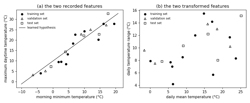
Fig. 1(a) draws the days at Krems this
way, with the hypothesis $\widehat{h}$ learned by
least squares on the $220$ training set days, and
Fig. 1(b) draws the same days after a
feature transformation.
pythondemos/scatterplot.py
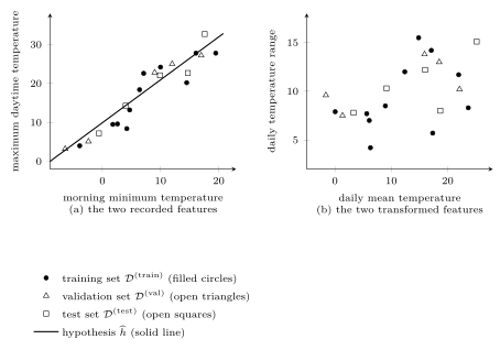
B-transformA feature transformation changes the picture, and the two pictures beside each other say what it did. Fig. 1(b) replaces the two recorded temperatures by the daily mean $(x_{1} + x_{2})/2$ and the daily range $x_{2} - x_{1}$, an invertible linear map. The elongated cloud becomes a cloud with no line through it: over all $366$ days the sample correlation coefficient falls from $0.88$ to $0.43$, and the daily mean alone carries $76.6$ percent of the sum of the two sample variances, against $39.0$ percent for the morning minimum. Keeping one of two features is the smallest dimensionality reduction, and a scatterplot is how its cost is judged by eye.
B-thinMarkers that nearly coincide hide each other, so a scatterplot stays legible only while it carries few of them. Of the $366$ days at Krems, $176$ lie within half a degree of another day and overlap at any legible marker size. A scatterplot therefore draws about twenty data points at most, chosen by a stated rule, while every number quoted beside it is computed from the whole dataset. The $21$ days of Fig. 1 are chosen this way, and no two of them lie within half a degree of each other; their sample correlation coefficient is $0.94$, close to the $0.88$ of all $366$ days.
B-plotA dataset with more than two features has no single scatterplot. One answer is a matrix of them, one panel for every pair of features (Hastie et al., 2009, Sect. 3.2.1), and another is a dimensionality reduction to two features, such as principal component analysis (PCA), after which the picture shows what survived the reduction. Neither answer is free. A matrix of panels grows with the square of the number of features, and it asks the reader to hold one panel against another. A reduction to two features draws the new features and not the recorded ones. What the scatterplot buys for that price is what a table of numbers withholds: a dataset a reader takes in at a glance. The device has outlived every change in how data are stored, and the first known scatterplot is Herschel's $1833$ plot of the position angle against the separation of double stars (Friendly and Denis, 2005).
See also: data point, dataset, feature, feature vector, label, hypothesis, training set, validation set, test set, outlier, cluster, feature transformation, dimensionality reduction, principal component analysis, correlation, histogram.
@misc{dictml_scatterplot,
  author = {Jung, Alexander},
  editor = {Olioumtsevits, Konstantina and Schnoor, Ekkehard},
  title = {scatterplot},
  howpublished = {Dictionary of Applied Machine Learning (course edition)},
  year = {2026},
  doi = {10.5281/zenodo.21569296},
  note = {ISBN 978-952-64-3013-3, CC BY 4.0, retrieved 2026-11-20},
  url = {https://dictionaryofml.org/terms/scatterplot.html}
}