B-plot writes when the script runsDictionary of Applied Machine Learning · scatterplot
Updated on 2026-11-19
Numerical companion to the entry scatterplot: it recomputes what the entry states and prints one line per check
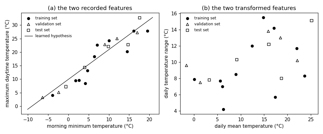
Numerical companion to the glossary entry 'scatterplot'. The 366 days of 2024 at Krems (GeoSphere station 3805) are data points. Each day carries the morning minimum temperature as its feature and the maximum daytime temperature as its label, so a scatterplot of the two puts one marker per day in the plane and a hypothesis that predicts the label from the feature is a curve in the same plane.
Run it without installing anything:uv run https://dictionaryofml.org/terms/scatterplot.py
uv downloads this script and the pinned NumPy and Matplotlib it needs, then runs it; the script fetches any input file it uses. To keep the output files, download scatterplot.py into a folder and run uv run scatterplot.py there. With NumPy and Matplotlib already installed, python3 scatterplot.py, from any directory — it writes its output files into the current directory. Fixed seeds, so the printed numbers reproduce exactly. Download scatterplot.py · Notebook · Open in Colab
Before running a downloaded copy, scan it: uvx bandit -q -t B102,B307,B602,B605 scatterplot.py (B102,B307,B602,B605 are the exec, eval and shell checks of bandit) reports nothing: the script runs no shell command and evaluates no generated code.
One cell per block of the script: the code, and what that code printed when it last ran here
"""The scatterplot of a dataset with two numeric features: the days of 2024
at Krems an der Donau drawn as markers, before and after a feature
transformation.

Purpose
-------
Numerical companion to the glossary entry 'scatterplot'.  The 366 days of
2024 at Krems (GeoSphere station 3805) are data points.  Each day carries
the morning minimum temperature as its feature and the maximum daytime
temperature as its label, so a scatterplot of the two puts one marker per
day in the plane and a hypothesis that predicts the label from the feature
is a curve in the same plane.

The demo turns what a reader sees in such a picture into numbers that can
be checked: the elongated cloud is a sample correlation coefficient close
to one and a leading principal direction that carries almost all of the
sample variance; the day that sits far below the learned line is the
largest absolute residual; and the same days drawn in the transformed
features (daily mean temperature, daily temperature range) form a cloud
whose spread is almost entirely along the first axis, which is what a
dimensionality reduction of these two features exploits.

It also measures the house rule on how many markers a scatterplot may
carry.  Of the 366 days, many lie within half a degree of another day and
their markers overlap at any readable marker size.  Keeping every 20th
training day and every 15th validation and test day leaves 21 days, a
picture in which far fewer markers overlap, while the sample correlation
coefficient of the drawn days stays close to the 366-day value, so the
thinned picture still shows what the full record shows.

Self-contained (numpy and matplotlib only), fixed seed for the split; the
GeoSphere download falls back to the committed CSV.

Blocks
------
[B-data]      Daily minimum and maximum temperature at Krems for 2024
              (366 days, no missing value).
[B-split]     A fixed-seed split of the 366 days into a training set, a
              validation set, and a test set.
[B-learn]     Least squares on the training set gives the linear
              hypothesis drawn as the solid line of panel (a).
[B-structure] The cloud of panel (a) as numbers: the sample correlation
              coefficient of the two features, the share of the sample
              variance along the leading principal direction, and the day
              with the largest absolute residual.
[B-transform] The same days in the transformed features (daily mean, daily
              range): the sample correlation coefficient falls and the
              spread concentrates on the first axis.
[B-thin]      The deterministic thinning rule for the figure, 21 of the
              366 days: how many markers overlap before and after the
              thinning, and that the sample correlation coefficient
              survives it.
[B-plot]      CSVs for the two panels and the matplotlib preview.

Outputs
-------
scatterplot_weather.csv    : date, tmin, tmax for 2024 (committed copy).
scatterplot_days_plot.csv  : the 21 drawn days with their two features,
                             their transformed features, and their split.
scatterplot_line.csv       : two points of the learned hypothesis.
scatterplot.png            : matplotlib preview (checking only).
"""

# /// script
# requires-python = ">=3.10"
# dependencies = ["matplotlib==3.10.7", "numpy==2.3.4"]
# ///

import json
import urllib.request
from pathlib import Path

import numpy as np
import matplotlib

matplotlib.use("Agg")
import matplotlib.pyplot as plt

OUT_DIR = Path(__file__).parent

report = []


def check(name, ok):
    report.append((name, bool(ok)))
    print(f"  [{'ok' if ok else 'FAIL'}] {name}")


def crowded(points, radius):
    """Number of points that lie within `radius` of another point."""
    diff = points[:, None, :] - points[None, :, :]
    near = np.sqrt((diff ** 2).sum(axis=2)) < radius
    np.fill_diagonal(near, False)
    return int(near.any(axis=1).sum())
Installed 11 packages in 97ms
Daily minimum and maximum temperature at Krems for 2024 (366 days, no missing value).
print("[B-data] daily minimum and maximum temperature at Krems, 2024")
URL = ("https://dataset.api.hub.geosphere.at/v1/station/historical/"
       "klima-v2-1d?parameters=tlmin,tlmax&station_ids=3805"
       "&start=2024-01-01&end=2024-12-31")
CSV = OUT_DIR / "scatterplot_weather.csv"
try:
    with urllib.request.urlopen(URL, timeout=120) as resp:
        payload = json.load(resp)
    params = payload["features"][0]["properties"]["parameters"]
    records = [(stamp[:10], lo, hi)
               for stamp, lo, hi in zip(payload["timestamps"],
                                        params["tlmin"]["data"],
                                        params["tlmax"]["data"])]
    with open(CSV, "w") as fh:
        fh.write("date,tmin,tmax\n")
        for day, lo, hi in records:
            fh.write(f"{day},{lo},{hi}\n")
    print(f"    downloaded {len(records)} days")
except OSError as err:
    print(f"    download failed ({err}); reading the committed CSV")
    rows = CSV.read_text().strip().splitlines()[1:]
    records = [(d, float(a), float(b))
               for d, a, b in (r.split(",") for r in rows)]

check("[B-data] 366 days for 2024", len(records) == 366)
check("[B-data] no day is missing a temperature",
      all(lo is not None and hi is not None for _, lo, hi in records))
dates = [d for d, _, _ in records]
x = np.array([lo for _, lo, _ in records], dtype=float)
y = np.array([hi for _, _, hi in records], dtype=float)
m = len(x)
[B-data] daily minimum and maximum temperature at Krems, 2024
    downloaded 366 days
  [ok] [B-data] 366 days for 2024
  [ok] [B-data] no day is missing a temperature
A fixed-seed split of the 366 days into a training set, a validation set, and a test set.
print("[B-split] fixed-seed split of the 366 days")
rng = np.random.default_rng(2024)
perm = rng.permutation(m)
m_train, m_val = 220, 73
split = np.empty(m, dtype=int)                 # 0 train, 1 val, 2 test
split[perm[:m_train]] = 0
split[perm[m_train:m_train + m_val]] = 1
split[perm[m_train + m_val:]] = 2
counts = [int((split == s).sum()) for s in (0, 1, 2)]
check(f"[B-split] {counts[0]} training days, {counts[1]} validation days, "
      f"{counts[2]} test days, {sum(counts)} in total",
      counts == [220, 73, 73] and sum(counts) == m)
[B-split] fixed-seed split of the 366 days
  [ok] [B-split] 220 training days, 73 validation days, 73 test days, 366 in total
Least squares on the training set gives the linear hypothesis drawn as the solid line of panel (a).
print("[B-learn] linear hypothesis learned on the training days")
tr = split == 0
A = np.column_stack([np.ones(int(tr.sum())), x[tr]])
w0, w1 = np.linalg.lstsq(A, y[tr], rcond=None)[0]


def h(xx):
    return w0 + w1 * xx


res = y - h(x)
trainerr = float(np.mean(res[tr] ** 2))
valerr = float(np.mean(res[split == 1] ** 2))
check(f"[B-learn] h(x) = {w0:.2f} + {w1:.3f} x; the average squared "
      f"deviation of a day from this line is {trainerr:.1f} on the training "
      f"days and {valerr:.1f} on the validation days",
      0.5 < w1 < 1.5 and trainerr > 0)
[B-learn] linear hypothesis learned on the training days
  [ok] [B-learn] h(x) = 9.93 + 1.101 x; the average squared deviation of a day from this line is 18.0 on the training days and 19.6 on the validation days
The cloud of panel (a) as numbers: the sample correlation coefficient of the two features, the share of the sample variance along the leading principal direction, and the day with the largest absolute residual.
print("[B-structure] the elongated cloud as numbers")
rho = float(np.corrcoef(x, y)[0, 1])
check(f"[B-structure] sample correlation coefficient of the two features "
      f"{rho:.3f}: the markers of the 366 days lie close to a rising line",
      rho > 0.8)
X = np.column_stack([x, y])
ev = np.sort(np.linalg.eigvalsh(np.cov(X, rowvar=False)))[::-1]
share = float(ev[0] / ev.sum())
check(f"[B-structure] the leading principal direction carries "
      f"{100 * share:.1f} percent of the sample variance of the two "
      f"features", share > 0.9)
far = int(np.argmax(np.abs(res)))
check(f"[B-structure] the largest absolute residual is {abs(res[far]):.1f} "
      f"degrees, on {dates[far]} (minimum {x[far]:.1f}, maximum "
      f"{y[far]:.1f}, prediction {h(x[far]):.1f})",
      abs(res[far]) > 3 * np.sqrt(trainerr) / 2)
[B-structure] the elongated cloud as numbers
  [ok] [B-structure] sample correlation coefficient of the two features 0.880: the markers of the 366 days lie close to a rising line
  [ok] [B-structure] the leading principal direction carries 94.3 percent of the sample variance of the two features
  [ok] [B-structure] the largest absolute residual is 10.8 degrees, on 2024-04-07 (minimum 7.1, maximum 28.5, prediction 17.7)
The same days in the transformed features (daily mean, daily range): the sample correlation coefficient falls and the spread concentrates on the first axis.
print("[B-transform] daily mean temperature and daily temperature range")
u = (x + y) / 2.0                              # daily mean temperature
v = y - x                                      # daily temperature range
rho_t = float(np.corrcoef(u, v)[0, 1])
check(f"[B-transform] sample correlation coefficient of the transformed "
      f"features {rho_t:.3f}, against {rho:.3f} for the recorded ones",
      abs(rho_t) < abs(rho))
share_rec = float(np.var(x) / (np.var(x) + np.var(y)))
share_u = float(np.var(u) / (np.var(u) + np.var(v)))
check(f"[B-transform] the daily mean temperature carries "
      f"{100 * share_u:.1f} percent of the sum of the two sample variances, "
      f"the daily range {100 * (1 - share_u):.1f} percent; the recorded "
      f"features split the same sum {100 * share_rec:.1f} to "
      f"{100 * (1 - share_rec):.1f}", share_u > share_rec)
check("[B-transform] the transformation is invertible: the recorded "
      "temperatures are recovered as u - v/2 and u + v/2",
      np.allclose(u - v / 2, x) and np.allclose(u + v / 2, y))
[B-transform] daily mean temperature and daily temperature range
  [ok] [B-transform] sample correlation coefficient of the transformed features 0.427, against 0.880 for the recorded ones
  [ok] [B-transform] the daily mean temperature carries 76.6 percent of the sum of the two sample variances, the daily range 23.4 percent; the recorded features split the same sum 39.0 to 61.0
  [ok] [B-transform] the transformation is invertible: the recorded temperatures are recovered as u - v/2 and u + v/2
The deterministic thinning rule for the figure, 21 of the 366 days: how many markers overlap before and after the thinning, and that the sample correlation coefficient survives it.
print("[B-thin] every 20th training day and every 15th validation and "
      "test day")
STRIDE = (20, 15, 15)
idx = np.sort(np.concatenate(
    [np.flatnonzero(split == s)[::STRIDE[s]] for s in (0, 1, 2)]))
drawn = [int((split[idx] == s).sum()) for s in (0, 1, 2)]
check(f"[B-thin] every 20th of the {counts[0]} training days, every 15th of "
      f"the {counts[1]} validation days, and every 15th of the {counts[2]} "
      f"test days: {drawn[0]} + {drawn[1]} + {drawn[2]} = {len(idx)} of the "
      f"{m} days are drawn", drawn == [11, 5, 5] and len(idx) == 21)
RADIUS = 0.5                                   # degrees
crowd_all = crowded(X, RADIUS)
crowd_thin = crowded(X[idx], RADIUS)
check(f"[B-thin] {crowd_all} of the {m} days lie within {RADIUS} degrees of "
      f"another day, so their markers overlap at any readable marker size; "
      f"{crowd_thin} of the {len(idx)} drawn days do", crowd_thin < crowd_all)
rho_thin = float(np.corrcoef(x[idx], y[idx])[0, 1])
check(f"[B-thin] sample correlation coefficient of the drawn days "
      f"{rho_thin:.3f}, within {abs(rho_thin - rho):.3f} of the {m}-day "
      f"value {rho:.3f}", abs(rho_thin - rho) < 0.1)
[B-thin] every 20th training day and every 15th validation and test day
  [ok] [B-thin] every 20th of the 220 training days, every 15th of the 73 validation days, and every 15th of the 73 test days: 11 + 5 + 5 = 21 of the 366 days are drawn
  [ok] [B-thin] 176 of the 366 days lie within 0.5 degrees of another day, so their markers overlap at any readable marker size; 0 of the 21 drawn days do
  [ok] [B-thin] sample correlation coefficient of the drawn days 0.944, within 0.064 of the 366-day value 0.880
CSVs for the two panels and the matplotlib preview.
print("[B-plot] CSVs for the two panels and the preview")
with open(OUT_DIR / "scatterplot_days_plot.csv", "w") as fh:
    fh.write("tmin,tmax,tmean,trange,split\n")
    for i in idx:
        fh.write(f"{x[i]:.1f},{y[i]:.1f},{u[i]:.2f},{v[i]:.2f},"
                 f"{split[i]}\n")
x_lo, x_hi = float(x.min()), float(x.max())
with open(OUT_DIR / "scatterplot_line.csv", "w") as fh:
    fh.write("tmin,pred\n")
    for xx in (x_lo, x_hi):
        fh.write(f"{xx:.2f},{h(xx):.3f}\n")

MARKS = ((0, "o", "k", "training set"),
         (1, "^", "none", "validation set"),
         (2, "s", "none", "test set"))
fig, (ax1, ax2) = plt.subplots(1, 2, figsize=(9.4, 3.9))
for s, mk, fc, lab in MARKS:
    sel = idx[split[idx] == s]
    ax1.scatter(x[sel], y[sel], marker=mk, facecolors=fc,
                edgecolors="black", s=28, label=lab)
    ax2.scatter(u[sel], v[sel], marker=mk, facecolors=fc,
                edgecolors="black", s=28, label=lab)
ax1.plot([x_lo, x_hi], [h(x_lo), h(x_hi)], "k-", lw=0.9,
         label="learned hypothesis")
ax1.set_xlabel("morning minimum temperature (°C)")
ax1.set_ylabel("maximum daytime temperature (°C)")
ax1.set_title("(a) the two recorded features")
ax1.legend(frameon=False, fontsize=8)
ax2.set_xlabel("daily mean temperature (°C)")
ax2.set_ylabel("daily temperature range (°C)")
ax2.set_title("(b) the two transformed features")
ax2.legend(frameon=False, fontsize=8)
fig.tight_layout()
fig.savefig(OUT_DIR / "scatterplot.png", dpi=110)

n_ok = sum(ok for _, ok in report)
print(f"\n{n_ok}/{len(report)} checks pass")
if n_ok != len(report):
    raise SystemExit(1)
[B-plot] CSVs for the two panels and the preview

13/13 checks pass
B-plot writes when the script runs