hardclustering.py, which recomputes what the entry states: the script block by block · open in ColabDictionary of Applied Machine Learning: 147 machine-learning terms, each with a definition, a figure, citations and a Python demo · All terms · Demos · Start here
Updated on 2026-11-19
Readiness 88/100
See also clustering cluster soft clustering degree of belonging cluster centroid clustering error $k$-means density-based spatial clustering of applications with noise spectral clustering graph clustering Gaussian mixture model expectation–maximization label classification unsupervised learning empirical risk minimization hypothesis training error accuracy $\bf 0/1$ loss confusion matrix
Hard clustering is the task of decomposing a dataset into a few clusters such that every data point belongs to exactly one cluster, so the clusters form a partition of the dataset. Its output is a cluster assignment, an index in $\{1, \ldots, k\}$ for every data point, which is a label-like quantity computed from the feature vectors alone and carries no meaning beyond the partition. Written as a one-hot vector, the assignment is a degree of belonging that is either $0$ or $1$, so hard clustering is the special case of soft clustering in which every vector of degrees of belonging is a vertex of the probability simplex. $k$-means delivers a hard clustering whose clusters are convex regions around cluster centroids, density-based spatial clustering of applications with noise (DBSCAN) one whose clusters are chains of densely surrounded data points, and spectral clustering one computed from eigenvectors of the Laplacian matrix of a similarity graph. A method that represents a cluster by a cluster centroid learns a hypothesis that assigns any feature vector to a cluster, and minimizing its clustering error is empirical risk minimization (ERM). A hard clustering is evaluated internally by the clustering error and externally against a reference partition, by the accuracy after the best renumbering of the clusters or by the Rand index, the fraction of pairs of data points that both partitions place together or apart.
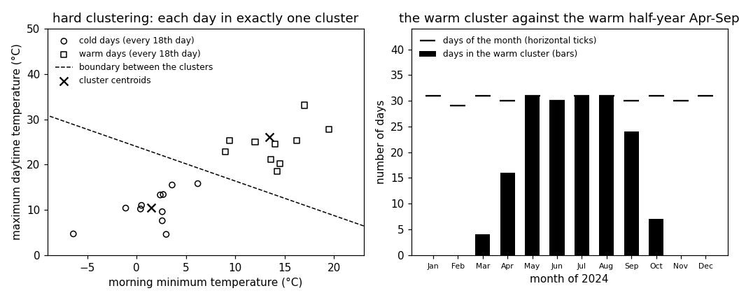
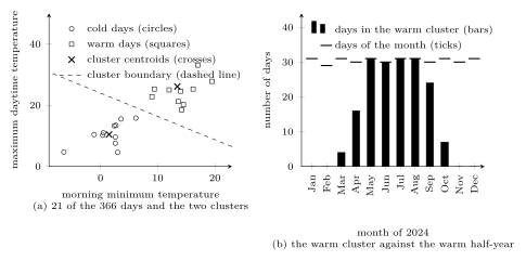
hardclustering.py, which recomputes what the entry states: the script block by block · open in ColabB-dataConsider the $366$ days of $2024$ at Krems an der Donau, each a data point with a feature vector ${\mathbf x} \in \mathbb{R}^{2}$ that holds the morning minimum and the maximum daytime temperature of the day. A heating utility that plans its fuel purchases by weather regime needs every day in exactly one regime. Hard clustering is the clustering task that delivers this: it decomposes the dataset into $k$ clusters such that every data point belongs to exactly one of them (Hastie et al., 2009, Sect. 14.3.5; Jain et al., 1999, Sect. 2; Shalev-Shwartz and Ben-David, 2014, Ch. 22). With $k = 2$, $k$-means splits the days into $192$ cold days and $174$ warm days (Fig. 1(a)); each day is a cold day or a warm day, never both and never neither.
B-partitionFormally, a hard clustering of a dataset $\mathcal{D} = \{{\mathbf x}^{(1)}, \ldots, {\mathbf x}^{(m)}\}$ consists of $k$ clusters $\mathcal{C}^{(1)}, \ldots, \mathcal{C}^{(k)} \subseteq \mathcal{D}$ that are disjoint and together cover the dataset, \begin{equation} \label{equ_hardclustering_partition_dict} \mathcal{C}^{(c)} \cap \mathcal{C}^{(c')} = \emptyset \text{ for } c \neq c' \quad \text{and} \quad \bigcup_{c=1}^{k} \mathcal{C}^{(c)} = \mathcal{D} \text{,} \end{equation} i.e., a partition of the dataset. The partition \(\eqref{equ_hardclustering_partition_dict}\) is the same object as the cluster assignment $\widehat{c}^{(r)} \in \{1, \ldots, k\}$ of each data point $r = 1, \ldots, m$, since $\mathcal{C}^{(c)} = \{{\mathbf x}^{(r)} : \widehat{c}^{(r)} = c\}$. The assignment is a label-like output. Like the label of a data point in classification, it takes one of finitely many values. Unlike a label, it is not given with the data but computed from the feature vectors alone, which makes hard clustering a form of unsupervised learning. The index $c$ of a cluster carries no meaning beyond the partition: renumbering the clusters yields the same hard clustering (Hastie et al., 2009, Sect. 14.3.5).
The assignment of data point $r$ can also be written as a vector of degrees of belonging $u_{c}^{(r)}$, one for each cluster, \begin{equation} \label{equ_hardclustering_onehot_dict} u_{c}^{(r)} := \begin{cases} 1 & \text{if } \widehat{c}^{(r)} = c \text{,} \\ 0 & \text{otherwise,} \end{cases} \qquad c = 1, \ldots, k \text{,} \end{equation} a one-hot vector with a single entry $1$ (Bishop, 2006, Sect. 9.1). A soft clustering method assigns to each data point a vector $\big(u_{1}^{(r)}, \ldots, u_{k}^{(r)}\big)^{\top}$ of nonnegative degrees of belonging that sum to one, i.e., a point of the probability simplex $\Delta^{k-1}$; a Gaussian mixture model (GMM), for example, uses the posterior distribution of the cluster index. Hard clustering is the special case in which every such vector is a vertex of the probability simplex, so each degree of belonging \(\eqref{equ_hardclustering_onehot_dict}\) is $0$ or $1$. A soft clustering is turned into a hard clustering by assigning each data point to the cluster with the largest degree of belonging (Jain et al., 1999, Sect. 5), and a GMM whose covariance matrices are all $\sigma^{2} \mathbf{I}$ delivers, as $\sigma^{2} \to 0$, the hard clustering of $k$-means (Bishop, 2006, Sect. 9.3.2).
B-boundaryHard clustering methods differ in how they represent a cluster. $k$-means represents cluster $c$ by a cluster centroid ${{\mathbf w}}^{(c)} \in \mathbb{R}^{d}$ and assigns each data point to the nearest one, $\widehat{c}^{(r)} = \mathop{\mathrm{arg\,min}}_{c = 1, \ldots, k} \left\lVert {\mathbf x}^{(r)} - {{\mathbf w}}^{(c)} \right\rVert_{2}$ (Lloyd, 1982; MacQueen, 1967). The feature vectors assigned to ${{\mathbf w}}^{(c)}$ form a convex region of the feature space bounded by hyperplanes, one for each other cluster centroid, namely the perpendicular bisector of the segment between the two cluster centroids. For the two cluster centroids at Krems, $(1.5, 10.5)$ and $(13.4, 26.1)$, this boundary is the dashed line of Fig. 1(a); the day nearest to it, March $28$, lies $0.22$ degrees from it. Density-based spatial clustering of applications with noise (DBSCAN) represents a cluster as a maximal set of data points connected through a chain of densely surrounded data points, so a cluster can have any shape and the number $k$ is an output rather than an input (Ester et al., 1996). Data points that belong to no such chain are noise, and the clusters of DBSCAN partition the dataset only after the noise points are removed or collected in a set of their own. Spectral clustering represents the data points as the nodes of a similarity graph, computes from $k$ eigenvectors of its Laplacian matrix a new feature vector in $\mathbb{R}^{k}$ for each node, and runs $k$-means on these new feature vectors (Luxburg, 2007, Sect. 4). The resulting clusters are convex regions in the new feature space but need not be convex in the original one.
A hard clustering method that represents a cluster by a cluster centroid learns a hypothesis: the map $h({\mathbf x}) = {{\mathbf w}}^{(c^{\star}({\mathbf x}))}$ that sends any feature vector to its nearest cluster centroid, with $c^{\star}({\mathbf x}) = \mathop{\mathrm{arg\,min}}_{c = 1, \ldots, k} \left\lVert {\mathbf x} - {{\mathbf w}}^{(c)} \right\rVert_{2}$. The partition \(\eqref{equ_hardclustering_partition_dict}\) of the dataset is the restriction of this map to the dataset, and a data point outside the dataset, say a day of $2025$, is assigned to the cluster of its nearest cluster centroid without recomputing the partition. Choosing the cluster centroids that minimize the clustering error, the average squared Euclidean distance between a data point and its cluster centroid, is empirical risk minimization (ERM) over the hypothesis space of all such maps. The clustering error is therefore the training error of the learned hypothesis, and it is the internal measure of a hard clustering, computed from the dataset alone. It falls as $k$ grows and vanishes when every data point is its own cluster, so it cannot choose $k$.
B-evalAn external measure compares the hard clustering with a reference partition of the same dataset, here the cold half-year from October to March ($183$ days) and the warm half-year from April to September ($183$ days). Since the cluster indices carry no meaning, the comparison must not depend on their numbering. One way is to renumber the clusters by the bijection onto the reference indices that maximizes the fraction of data points on which the two partitions agree. This fraction is the accuracy of the renumbered hard clustering, one minus its average $0/1$ loss against the reference indices, and the table of counts behind it is a confusion matrix. At Krems, $172$ of the $192$ cold days fall into the cold half-year and $163$ of the $174$ warm days into the warm half-year, an accuracy of $91.5$ percent. The disagreement is concentrated in four months (Fig. 1(b)): January, February, November, and December lie entirely in the cold cluster, May to August entirely in the warm one, and the days of March, April, September, and October are split.
B-seasonsThe other way counts pairs of data points. Let $a$ be the
number of pairs that both partitions place in one cluster
and $e$ the number that both place in different clusters.
The Rand index is
\begin{equation}
\label{equ_hardclustering_rand_dict}
\frac{a + e}{\binom{m}{2}} \text{,}
\end{equation}
the fraction of pairs on which the partitions agree
(Murphy, 2012, Sect. 25.1.2; Rand, 1971). It is
$1$ for identical partitions and unchanged by renumbering, since
it never reads an index. Of the $66795$ pairs of days at Krems,
$28154$ are together and $28256$ apart in both partitions, a
Rand index \(\eqref{equ_hardclustering_rand_dict}\) of $0.845$. An
adjusted Rand index subtracts the value expected for two
independent random partitions with the same cluster sizes
(Hubert and Arabie, 1985). A reference partition is a standard
set by the application, not a property of the feature vectors.
With $k = 4$ clusters against the four seasons,
the accuracy after renumbering drops to $59.6$ percent and
the Rand index to $0.741$. Spring and autumn days have the same
temperatures: the cluster that holds most spring days
consists of $55$ percent spring days and $25$ percent autumn
days. In
image segmentation, a hard clustering of the pixels of a
photograph by color assigns every pixel to exactly one region,
and its evaluation against a hand-drawn segmentation uses the
same two measures.
pythondemos/hardclustering.py
See also: clustering, cluster, soft clustering, degree of belonging, cluster centroid, clustering error, $k$-means, Lloyd's algorithm, density-based spatial clustering of applications with noise, spectral clustering, graph clustering, Gaussian mixture model, expectation–maximization, probability simplex, label, classification, unsupervised learning, empirical risk minimization, hypothesis, training error, accuracy, $\bf 0/1$ loss, confusion matrix, image segmentation.
@misc{dictml_hardclustering,
  author = {Jung, Alexander},
  editor = {Olioumtsevits, Konstantina and Schnoor, Ekkehard},
  title = {hard clustering},
  howpublished = {Dictionary of Applied Machine Learning (course edition)},
  year = {2026},
  doi = {10.5281/zenodo.21569296},
  note = {ISBN 978-952-64-3013-3, CC BY 4.0, retrieved 2026-11-20},
  url = {https://dictionaryofml.org/terms/hardclustering.html}
}