dob.py, which recomputes what the entry states: the script block by block · open in ColabDictionary of Applied Machine Learning: 147 machine-learning terms, each with a definition, a figure, citations and a Python demo · All terms · Demos · Start here
Updated on 2026-11-19
Readiness 88/100
See also cluster clustering soft clustering hard clustering cluster centroid Gaussian mixture model expectation–maximization $k$-means clustering error
A degree of belonging is a number that indicates the extent to which a data point belongs to a cluster, one for each pair of a data point and a cluster of a clustering. In the most common formulation, the degrees of belonging of one data point are nonnegative and sum to one, so they form a vector of the probability simplex and a probability mass function (pmf) over the cluster indices. Hard clustering is the special case in which this vector has one entry equal to one and all others equal to zero, as delivered by $k$-means. A principled construction of degrees of belonging strictly between zero and one is the posterior distribution of the cluster index under a Gaussian mixture model (GMM), which the expectation–maximization (EM) algorithm computes in its E-step. The degrees of belonging in turn determine the clusters: the mean of a cluster is the average of the feature vectors weighted by them, and with degrees of belonging of zero or one this weighted average is the averaging step of Lloyd's algorithm. As the common variance of the clusters of a GMM shrinks to zero, the degrees of belonging turn into zero or one and soft clustering turns into hard clustering.
dob.py, which recomputes what the entry states: the script block by block · open in ColabB-hardConsider the $366$ days of one
year at Krems an der Donau, each a data point with a
feature vector ${\mathbf x} \in \mathbb{R}^{2}$ that holds the
morning minimum and the maximum daytime temperature of the day.
A clustering method decomposes these days into a cold
cluster and a warm cluster. A day in January is a cold
day and a day in July a warm day, but 28 May 2024, with a morning
minimum of $11.1$ and a maximum of $21.3$ degrees, lies between
the two. A degree of belonging $u_{c}^{(r)}$
is a number that indicates the extent to which data point
$r$ belongs to cluster $c$, for
$c = 1, \ldots, k$ and $r = 1,
\ldots, m$. For 28 May 2024, the Gaussian mixture model (GMM) of
Fig. 2 delivers the degrees of belonging
$0.50$ to the cold and $0.50$ to the warm cluster, while a
day in January obtains $1.00$ and $0.00$. In the most common
formulation, the degrees of belonging of one data point are
nonnegative and sum to one (Bezdek, 1981;
Ruspini, 1969),
\begin{equation}
\label{equ_dob_simplex_dict}
u_{c}^{(r)} \geq 0
\quad \text{for } c = 1, \ldots, k
\qquad \text{and} \qquad
\sum_{c=1}^{k} u_{c}^{(r)}
= 1 \text{.}
\end{equation}
The vector
${\mathbf u}^{(r)} := \big(u_{1}^{(r)}, \ldots,
u_{k}^{(r)}\big)^{\top}$ then lies in the
probability simplex $\Delta^{k-1}$. It is the
probability mass function (pmf) of a random variable (RV) with values in $\{1, \ldots, k\}$,
the cluster index of the data point. Possibilistic
clustering drops the sum constraint of the simplex
condition \(\eqref{equ_dob_simplex_dict}\) and lets each degree of
belonging vary in $[0, 1]$ on its own (Krishnapuram and Keller, 1993).
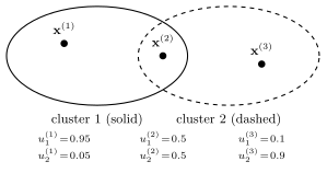
Fig. 1 sketches three
data points and their degrees of belonging to two
overlapping clusters.
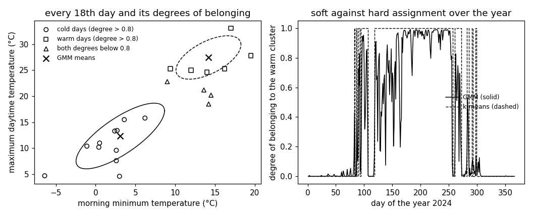
B-gmmSoft clustering methods assign a data point to several clusters with degrees of belonging strictly between $0$ and $1$. A principled construction uses a probabilistic model for the data points, the GMM. Under it, the cluster index $I^{(r)} \in \{1, \ldots, k\}$ of data point $r$ is an unobserved RV with $\mathbb{P}\left(I^{(r)} = c\right) = p_{c}$. Given $I^{(r)} = c$, the feature vector ${\mathbf x}^{(r)}$ is drawn from a multivariate normal distribution with mean ${\boldsymbol \mu}^{(c)}$ and covariance matrix $\mathbf{C}^{(c)}$. The degree of belonging is then the posterior distribution of the cluster index given the observed feature vector, \begin{equation} \label{equ_dob_gmm_dict} u_{c}^{(r)} := \mathbb{P}\left(I^{(r)} = c \mid {\mathbf x}^{(r)}\right) = \frac{p_{c}\, \mathcal{N}\left({\boldsymbol \mu}^{(c)},\mathbf{C}^{(c)}\right)({\mathbf x}^{(r)})} {\sum_{c'=1}^{k} p_{c'}\, \mathcal{N}\left({\boldsymbol \mu}^{(c')},\mathbf{C}^{(c')}\right)({\mathbf x}^{(r)})}\text{,} \end{equation} the responsibility of cluster $c$ for the data point (Bishop, 2006, Sect. 9.2; Murphy, 2012, Sect. 11.2.3). The posterior degrees of belonging \(\eqref{equ_dob_gmm_dict}\) are the probabilities of the $k$ values of one RV, so they satisfy the simplex condition \(\eqref{equ_dob_simplex_dict}\) by construction. The model parameters $p_{c}$, ${\boldsymbol \mu}^{(c)}$, and $\mathbf{C}^{(c)}$ of the GMM are learned by maximum likelihood. This is an instance of empirical risk minimization (ERM): the loss of a data point is the negative logarithm of the probability density function (pdf) of the GMM at its feature vector, and the clustering error is the average of this loss over the dataset. For the days at Krems, a two-component GMM learned by the expectation–maximization (EM) algorithm has the means $(3.1, 12.3)$ and $(14.2, 27.5)$ and the cluster probabilities $0.63$ and $0.37$. Under it, $58$ of the $366$ days have no degree of belonging above $0.8$, $23$ of them in May and none between November and February (Fig. 2).
B-centroidThe degrees of belonging determine the clusters in turn. In the M-step of the EM algorithm, the mean of cluster $c$ is the average of the feature vectors weighted by the degrees of belonging. The cluster probability is the average of the degrees of belonging themselves. In formulas, \begin{equation} \label{equ_dob_centroid_dict} {\boldsymbol \mu}^{(c)} = \frac{\sum_{r=1}^{m} u_{c}^{(r)}\, {\mathbf x}^{(r)}} {\sum_{r=1}^{m} u_{c}^{(r)}} \qquad \text{and} \qquad p_{c} = \frac{1}{m} \sum_{r=1}^{m} u_{c}^{(r)} \quad \text{for } c = 1, \ldots, k\text{.} \end{equation} The covariance matrix $\mathbf{C}^{(c)}$ is the covariance matrix of the feature vectors under the same weighting (Bishop, 2006, Sect. 9.2.2). A day with the degrees of belonging $0.50$ and $0.50$ counts half towards each mean. With the degrees of belonging \(\eqref{equ_dob_hard_dict}\) of a hard clustering, the weighted average \(\eqref{equ_dob_centroid_dict}\) is the mean of the data points assigned to cluster $c$, which is the averaging step of Lloyd's algorithm for $k$-means, and $p_{c}$ is the share of data points in that cluster. The EM algorithm alternates the posterior \(\eqref{equ_dob_gmm_dict}\) with the weighted averages \(\eqref{equ_dob_centroid_dict}\), so the degrees of belonging are recomputed in every iteration: they are not model parameters but a function of the model parameters and of the feature vector. At the fixed point of the EM algorithm on the days at Krems, each mean equals the average of the days weighted by their degrees of belonging and differs from the $k$-means cluster centroid of the same cluster by at most $1.9$ degrees.
B-limitHard clustering is also a limit of the posterior degrees of belonging \(\eqref{equ_dob_gmm_dict}\). Fix every cluster probability at $1/k$ and every covariance matrix at $\sigma^{2} \mathbf{I}$, a multiple of the identity matrix $\mathbf{I}$ with one common variance $\sigma^{2}$. The posterior \(\eqref{equ_dob_gmm_dict}\) then depends on ${\mathbf x}^{(r)}$ only through its squared Euclidean distances to the means. As $\sigma^{2}$ shrinks towards $0$, it concentrates on the nearest mean: every degree of belonging tends to $0$ or $1$, and the EM algorithm reduces to Lloyd's algorithm (Bishop, 2006, Sect. 9.3.2; Hastie et al., 2009, Sect. 14.3.7). For the days at Krems, with the two $k$-means cluster centroids as means and $\sigma^{2} = 1$, no day has both degrees of belonging above $0.2$, and every degree of belonging is within $0.01$ of its $k$-means value \(\eqref{equ_dob_hard_dict}\). With $\sigma^{2} = 50$, $16$ percent of the days have both degrees above $0.2$. With $\sigma^{2} = 1000$, every day has both above $0.2$ and no degree of belonging exceeds $0.63$.
B-plotThe degrees of belonging of a data point are the value of a
hypothesis at its feature vector. The posterior
\(\eqref{equ_dob_gmm_dict}\) is a map
$h: \mathbb{R}^{d} \rightarrow \Delta^{k-1}$
determined by the model parameters of the GMM, and the
assignment rule of $k$-means is a map from
$\mathbb{R}^{d}$ to the vertices of
$\Delta^{k-1}$ determined by the
cluster centroids. Either map applies to a day that did not
belong to the dataset the clusters were learned
from, which is how a clustering generalizes. A
hard clustering is derived from degrees of belonging by
assigning each data point to the cluster with the
largest one, and $1 - \max_{c = 1, \ldots, k}
u_{c}^{(r)}$ measures how uncertain that
assignment is (Murphy, 2012, Sect. 11.2.3). For the days at
Krems, the largest posterior degree of belonging names the
$k$-means cluster on $91.5$ percent of the days. In
medical image segmentation, the degrees of belonging of a
pixel to the tissue types let a pixel at the boundary between
two tissues belong partly to both, where a hard clustering
must pick one (Pham et al., 2000).
pythondemos/dob.py
Synonyms: membership degree, responsibility.
See also: cluster, clustering, soft clustering, hard clustering, cluster centroid, Gaussian mixture model, expectation–maximization, $k$-means, Lloyd's algorithm, posterior distribution, probability simplex, probability mass function, clustering error.
@misc{dictml_dob,
  author = {Jung, Alexander},
  editor = {Olioumtsevits, Konstantina and Schnoor, Ekkehard},
  title = {degree of belonging},
  howpublished = {Dictionary of Applied Machine Learning (course edition)},
  year = {2026},
  doi = {10.5281/zenodo.21569296},
  note = {ISBN 978-952-64-3013-3, CC BY 4.0, retrieved 2026-11-20},
  url = {https://dictionaryofml.org/terms/dob.html}
}