LapMat.py, which recomputes what the entry states: the script block by block · open in ColabDictionary of Applied Machine Learning: 147 machine-learning terms, each with a definition, a figure, citations and a Python demo · All terms · Demos · Start here
Updated on 2026-11-19
Readiness 88/100
See also weighted graph edge weight matrix eigenvalue eigenvector eigenvalue decomposition spectral clustering graph clustering regularization
The Laplacian matrix of a weighted graph with $n$ nodes is the $n \times n$ matrix ${\mathbf L}^{(\mathcal{G})} = {\mathbf D}^{(\mathcal{G})} - {\mathbf A}^{(\mathcal{G})}$, the degree matrix minus the adjacency matrix of the edge weights. Its quadratic form ${\mathbf x}^{\top} {\mathbf L}^{(\mathcal{G})} {\mathbf x}$ is the sum, over the edges, of the edge weight times the squared difference of the two entries of ${\mathbf x}$ at the ends of the edge. The Laplacian matrix is therefore a symmetric matrix and positive semi-definite (psd), the constant vector is an eigenvector with eigenvalue $0$, and the multiplicity of the eigenvalue $0$ equals the number of connected components of the graph. Two normalized variants divide the edge weights by the node degrees; they share their eigenvalues, which lie between $0$ and $2$. In machine learning (ML), the quadratic form is the penalty term of Laplacian regularization, which makes the values learned at connected nodes similar and predicts the value at an unlabeled node as the weighted average of its neighbors. The eigenvectors of its smallest eigenvalues are the coordinates that spectral clustering feeds to $k$-means.
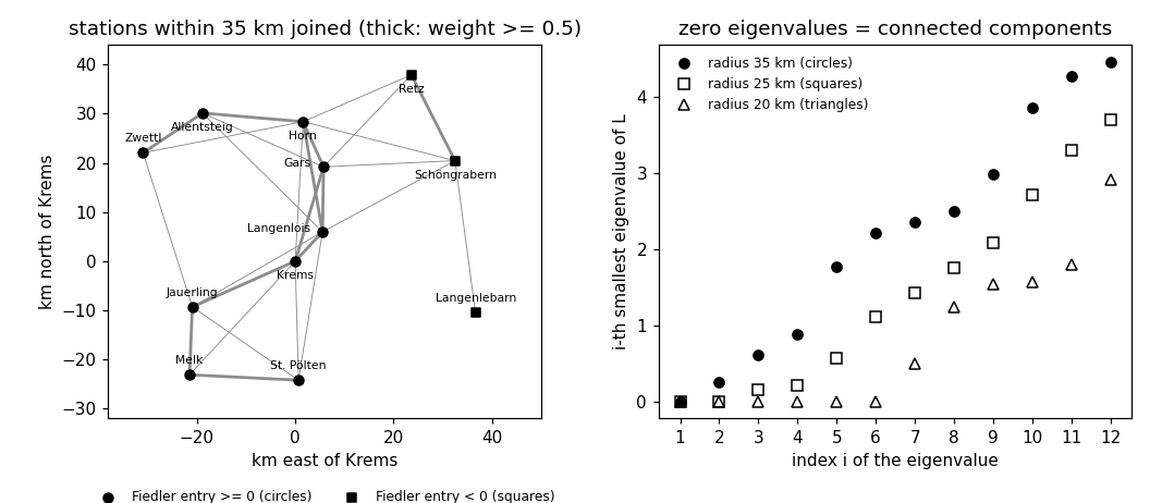
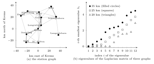
LapMat.py, which recomputes what the entry states: the script block by block · open in ColabB-dataTwelve weather stations around Krems an der Donau, from Melk and Zwettl in the west to Retz and Langenlebarn in the east, each recorded a mean temperature for the year $2024$: $12.6$ degrees Celsius at Krems, $9.6$ on the Jauerling mountain. Two stations at most $35$ km apart are joined by an edge whose weight decays with their distance, so the stations form a weighted graph $\mathcal{G}$ with $27$ edges (Fig. 2(a)). How much does the temperature vary along the edges of $\mathcal{G}$? One answer is the sum, over the edges, of the edge weight times the squared difference of the two temperatures at its ends. The Laplacian matrix of $\mathcal{G}$ is the matrix that computes this sum as a quadratic form in the vector of the twelve temperatures.
B-graphConsider an undirected graph $\mathcal{G} = \left( \mathcal{V},\mathcal{E} \right)$
with nodes $\mathcal{V} = \{1, \ldots, n\}$ and nonnegative
edge weights $A_{i,i'} =
A_{i',i}$, where
$A_{i,i'} = 0$ when $\mathcal{G}$ has no edge
$\{i,i'\}$ (Luxburg, 2007, Sect. 2.1). The
edge weights are the entries of the adjacency matrix
${\mathbf A}^{(\mathcal{G})} \in \mathbb{R}^{n \times n}$, and the
node degree $d^{(i)} :=
\sum_{i'=1}^{n} A_{i,i'}$
of node $i$ is the sum of the weights of its edges. The
Laplacian matrix of $\mathcal{G}$ is the difference
\begin{equation}
\label{equ_LapMat_def_dict}
{\mathbf L}^{(\mathcal{G})} := {\mathbf D}^{(\mathcal{G})} - {\mathbf A}^{(\mathcal{G})}
\text{, with the degree matrix } {\mathbf D}^{(\mathcal{G})} :=
\operatorname{diag}\big\{ d^{(1)}, \ldots,
d^{(n)} \big\} \text{.}
\end{equation}
The diagonal entry $L^{(\mathcal{G})}_{i,i}$ of
the Laplacian matrix \(\eqref{equ_LapMat_def_dict}\) is the
node degree $d^{(i)}$, and the off-diagonal
entry $L^{(\mathcal{G})}_{i,i'}$ is the negated
edge weight $-A_{i,i'}$, so every row
sums to zero (Hastie et al., 2009, Sect. 14.5.3;
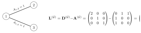
Luxburg, 2007, Sect. 3.1). Fig. 1
carries out the construction for a graph with three nodes
and two edges. For the station graph, the edge between Krems
and Langenlois, $8$ km apart, has weight $0.92$, the longest edges
have weight $0.23$, and Krems has degree $3.18$ from its six
neighbors.
B-eigenvaluesThree properties of the Laplacian matrix follow from the
quadratic form \(\eqref{equ_LapMat_quadform_dict}\)
(Luxburg, 2007, Prop. 1, Prop. 2; Mohar, 1991).
First, ${\mathbf L}^{(\mathcal{G})}$ is a
symmetric matrix and positive semi-definite (psd), since every term of the sum
is nonnegative, so its eigenvalues are real and can be
ordered as $0 \leq \lambda_{1} \leq \lambda_{2} \leq \ldots \leq
\lambda_{n}$. Second, the constant vector
$\mathbf{1} = (1, \ldots, 1)^{\top}$ makes every term vanish, and
${\mathbf L}^{(\mathcal{G})} \mathbf{1} = \mathbf{0}$ since every row sums to
zero, so $\lambda_{1} = 0$ with the eigenvector $\mathbf{1}$.
Third, the multiplicity of the eigenvalue $0$ equals the
number of connected components of $\mathcal{G}$. A vector
${\mathbf x}$ with ${\mathbf x}^{\top} {\mathbf L}^{(\mathcal{G})} {\mathbf x} = 0$ takes the same
value at the two ends of every edge, so it is constant on each
component, and the indicator vectors of the components
span the nullspace of ${\mathbf L}^{(\mathcal{G})}$. The station
graph is connected, so $\lambda_{1} = 0$ is simple and
$\lambda_{2} = 0.25$ is positive. Joining only stations at most
$25$ km apart leaves Langenlebarn without an edge and the
graph with two components, and the limit $20$ km leaves six
components; the eigenvalue $0$ then has multiplicity two
and six (Fig. 2(b)). The
second-smallest eigenvalue $\lambda_{2}$ is the
algebraic connectivity of $\mathcal{G}$, and the eigenvector of
$\lambda_{2}$ is the Fiedler vector (Fiedler, 1973). The
signs of its entries split the nodes into two clusters with
few edges between them (Fiedler, 1975). For the station
graph, the three stations more than $20$ km east of Krems,
Langenlebarn, Schöngrabern, and Retz, have negative entries and
the other nine have positive entries.
pythondemos/LapMat.py
In machine learning (ML), the Laplacian matrix enters through its quadratic form \(\eqref{equ_LapMat_quadform_dict}\) as a penalty term. Consider data points that are the nodes of $\mathcal{G}$, which is then a similarity graph, with a label $y_{i}$ known only for the nodes in a subset $\mathcal{A} \subset \mathcal{V}$. Examples are the stations with a record, or the users of a social network who filled in a profile field. A hypothesis is a vector ${\mathbf x} \in \mathbb{R}^{n}$ that assigns one value to every node, and the hypothesis space is $\mathbb{R}^{n}$. Laplacian regularization adds the quadratic form to the average squared error loss on the labeled nodes, \begin{equation} \label{equ_LapMat_reg_dict} \min_{{\mathbf x} \in \mathbb{R}^{n}} \frac{1}{|\mathcal{A}|} \sum_{i \in \mathcal{A}} \big( x_{i} - y_{i} \big)^{2} + \alpha \, {\mathbf x}^{\top} {\mathbf L}^{(\mathcal{G})} {\mathbf x} \text{,} \end{equation} with a hyperparameter $\alpha > 0$ (Belkin et al., 2004; Zhou and Schölkopf, 2004). Adding a penalty term is one of the three routes that regularization distinguishes, and this one implements the assumption that nodes joined by a heavy edge carry similar values. The training error alone says nothing about a node outside $\mathcal{A}$; the penalty term is the only term that constrains its value, so the generalization from the labeled to the unlabeled nodes comes from the edges. The objective \(\eqref{equ_LapMat_reg_dict}\) is convex and its minimizer solves a linear system, since the gradient of the quadratic form is $2 {\mathbf L}^{(\mathcal{G})} {\mathbf x}$. As $\alpha \to 0$, the minimizer pins $x_{i} = y_{i}$ on the labeled nodes and minimizes the quadratic form over the remaining entries. The entry of ${\mathbf L}^{(\mathcal{G})} {\mathbf x}$ at an unlabeled node is then zero. Such a node takes the weighted average of its neighbors, $x_{i} = (1/d^{(i)}) \sum_{i'=1}^{n} A_{i,i'} x_{i'}$, which is the harmonic solution of Zhu et al. (2003).
B-regularizeLeaving each station of Fig. 2(a) out in turn and predicting its mean temperature by this average of its neighbors gives a mean absolute error of $0.86$ degrees. Predicting the mean of the other eleven stations instead gives $1.12$ degrees. The largest error is at Jauerling, $955$ m above sea level, predicted at $12.3$ degrees against $9.6$ recorded. The edge weights encode distance but not altitude, so the penalty asks a mountain station to resemble the valley stations around it. The same quadratic form, with the model parameters of local models in place of the scalars $x_{i}$, is the generalized total variation (GTV) that generalized total variation minimization (GTVMin) penalizes in federated learning (FL). The eigenvectors of the smallest eigenvalues of a Laplacian matrix are the coordinates that spectral clustering hands to $k$-means (Luxburg, 2007, Sect. 4).
See also: graph, weighted graph, edge weight, adjacency matrix, node degree, matrix, positive semi-definite, eigenvalue, eigenvector, eigenvalue decomposition, connected, algebraic connectivity, Fiedler vector, spectral clustering, graph clustering, similarity graph, regularization, penalty term, generalized total variation, generalized total variation minimization.
@misc{dictml_LapMat,
  author = {Jung, Alexander},
  editor = {Olioumtsevits, Konstantina and Schnoor, Ekkehard},
  title = {Laplacian matrix},
  howpublished = {Dictionary of Applied Machine Learning (course edition)},
  year = {2026},
  doi = {10.5281/zenodo.21569296},
  note = {ISBN 978-952-64-3013-3, CC BY 4.0, retrieved 2026-11-20},
  url = {https://dictionaryofml.org/terms/LapMat.html}
}