graphclustering.py, which recomputes what the entry states: the script block by block · open in ColabDictionary of Applied Machine Learning: 147 machine-learning terms, each with a definition, a figure, citations and a Python demo · All terms · Demos · Start here
Updated on 2026-11-19
Readiness 88/100
See also clustering cluster weighted graph edge weight Laplacian matrix eigenvector spectral clustering $k$-means unsupervised learning
Graph clustering decomposes the nodes of a weighted graph, one node per data point, into clusters: subsets of nodes with a large total edge weight inside and a small total edge weight to the rest. Each edge weight expresses the similarity of two data points. The graph is either a similarity graph built from feature vectors, such as a $k$-nearest-neighbor graph ($k$-NN graph), or given by the application, such as papers joined by citations or users joined by friendships. The cut of a cluster is the total edge weight of the edges leaving it, and the ratio cut of a clustering is the sum of the cuts of its clusters, each divided by the number of nodes in the cluster, which keeps a single node from being split off. Finding the partition with the smallest ratio cut is computationally hard, so spectral clustering approximates it through eigenvectors of the Laplacian matrix, flow-based clustering through network flows, and convex clustering through a penalty term weighted by the edge weights. Applications include image segmentation, with pixels as nodes, and the detection of communities in social networks.
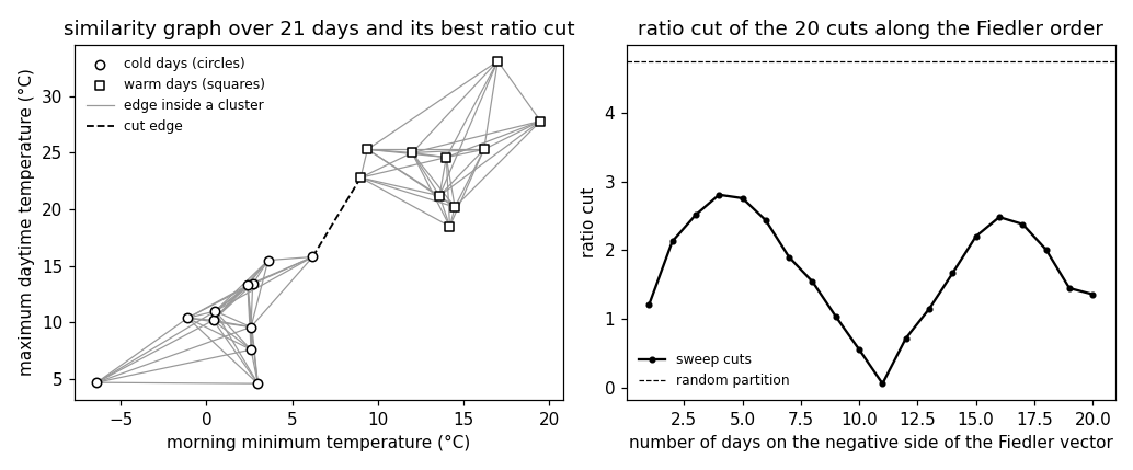
graphclustering.py, which recomputes what the entry states: the script block by block · open in ColabB-dataConsider every $18$th day of $2024$ at Krems an der Donau, $21$ days in all, each a data point with a feature vector ${\mathbf x} \in \mathbb{R}^{2}$ that holds the morning minimum and the maximum daytime temperature. Instead of measuring how far apart two days are, record which days are similar. Each day is a node of a graph, and two days are joined by an edge if one is among the six nearest neighbors of the other. The edge carries an edge weight between $0$ and $1$ that is close to $1$ for days with almost the same temperatures (Fig. 1(a)). Graph clustering decomposes the nodes of such a graph into clusters: subsets of nodes with a large total edge weight inside and a small total edge weight to the rest of the graph. For the $21$ days, the two clusters are $11$ cold days and $10$ warm days, joined by a single edge.
B-graphThe graph is built from feature vectors, as a similarity graph such as the $k$-nearest-neighbor graph ($k$-NN graph) with Gaussian edge weights (Hastie et al., 2009, Sect. 14.5.3; Luxburg, 2007, Sect. 2), or it is given by the application: scientific papers joined by citations, users of a social network joined by friendships, or web pages joined by links. In the second case the data points need no feature vectors at all, which is the main reason for clustering a graph rather than a feature space.
B-cutFormally, the data points are the nodes $i = 1, \ldots, m$ of a weighted graph $\mathcal{G}$ that is an undirected graph with the edge weights $A_{i,i'} = A_{i',i} \geq 0$, where $A_{i,i'} = 0$ means that the nodes $i$ and $i'$ are not joined by an edge. The cut of a cluster $\mathcal{C} \subseteq \{1, \ldots, m\}$ is the total edge weight of the edges that leave it, \begin{equation} \label{equ_graphclustering_cut_dict} \operatorname{cut}(\mathcal{C}) := \sum_{i \in \mathcal{C}} \, \sum_{i' \notin \mathcal{C}} A_{i,i'} \text{.} \end{equation} The cut \(\eqref{equ_graphclustering_cut_dict}\) of a single node is its node degree $d^{(i)} = \sum_{i'=1}^{m} A_{i,i'}$. For a vector ${\mathbf s} \in \{-1, 1\}^{m}$ with $s_{i} = 1$ for $i \in \mathcal{C}$ and $s_{i} = -1$ otherwise, the cut is the quadratic form $\operatorname{cut}(\mathcal{C}) = (1/4) \, {\mathbf s}^{\top} {\mathbf L}^{(\mathcal{G})} {\mathbf s}$ of the Laplacian matrix ${\mathbf L}^{(\mathcal{G})}$ (Luxburg, 2007, Sect. 5.1). A clustering into $k$ clusters $\mathcal{C}^{(1)}, \ldots, \mathcal{C}^{(k)}$ assigns each node to exactly one of them, and the sum of their cuts counts every edge between two clusters twice. Choosing the clusters to minimize this sum alone often splits off a single node (Luxburg, 2007, Sect. 5). For the $21$ days, the smallest cut over all $2^{20}$ two-way partitions is $0.32$, for the cold and the warm days, but the second smallest, $1.15$, already splits off the single day $26$ December, the day with the smallest node degree.
B-ratiocutThe ratio cut divides the cut of each cluster by its number of nodes (Hagen and Kahng, 1992), \begin{equation} \label{equ_graphclustering_ratiocut_dict} \sum_{c=1}^{k} \frac{\operatorname{cut}(\mathcal{C}^{(c)})} {|\mathcal{C}^{(c)}|} \text{.} \end{equation} A small cluster is charged a large share of its cut, so the ratio cut \(\eqref{equ_graphclustering_ratiocut_dict}\) favors clusters of similar size. The normalized cut divides by the total node degree of the cluster instead (Shi and Malik, 2000), so that a cluster is measured by its edge weights rather than by its number of nodes (Luxburg, 2007, Sect. 5). For the $21$ days, the smallest ratio cut over all two-way partitions is $0.061$, again for the cold and the warm days. Splitting off $26$ December has the ratio cut $1.21$, $20$ times as much. Ranked by the cut, this split was the second best partition; ranked by the ratio cut, it is the $54$th. A random partition into $11$ and $10$ days cuts $43$ of the $80$ edges, with the cut $24.9$ and the ratio cut $4.75$. Over all $167960$ partitions of these sizes, the ratio cut averages $4.67$. Finding a partition with the smallest ratio cut or normalized cut is computationally hard (Luxburg, 2007, Sect. 5). For $21$ nodes every partition can be enumerated, for the $12288$ patches of a photograph it cannot.
B-spectralGraph clustering methods differ in how they approximate a minimizer. Spectral clustering relaxes the constraint that each node is assigned to one cluster and solves the relaxed problem through eigenvectors of the Laplacian matrix (Luxburg, 2007, Sect. 5; Ng et al., 2001). For the ratio cut \(\eqref{equ_graphclustering_ratiocut_dict}\) of a connected graph and $k = 2$, the relaxed minimizer is the Fiedler vector (Fiedler, 1973), the eigenvector of the second smallest eigenvalue, the algebraic connectivity. The nodes are then split by the signs of its entries or at the best of the $m - 1$ thresholds along its sorted entries. For the $21$ days, whose graph is connected, the Fiedler vector is negative on the $11$ cold days and positive on the $10$ warm days, and the best of the $20$ thresholds returns the exact minimizer of the ratio cut (Fig. 1(b)). Flow-based clustering builds a feature vector for each node from network flows between selected nodes and applies $k$-means to these feature vectors (SarcheshmehPour et al., 2021). Convex clustering uses both the graph and the feature vectors of the nodes. It gives each node its own cluster centroid and adds a penalty term, weighted by the edge weights, that pulls the cluster centroids of joined nodes together until they coincide (Hocking et al., 2011). The nodes that share a cluster centroid form a cluster.
Graph clustering is unsupervised learning: the nodes carry no labels, and the hypothesis learned is the assignment of each node to a cluster index. The cut \(\eqref{equ_graphclustering_cut_dict}\) is a sum over the edges rather than over the data points. An edge costs its edge weight when its two nodes are assigned to different clusters and nothing otherwise, so the cut is the generalized total variation (GTV) of the assignment for the discrepancy that is $1$ for two different indices and $0$ for equal ones. Without the denominator of the ratio cut \(\eqref{equ_graphclustering_ratiocut_dict}\), assigning all but one node to the same cluster would be the cheapest choice, in the way that a training error of zero is reached by a hypothesis that is useless elsewhere.
B-plotA photograph is clustered into regions by graph clustering
with the pixels as nodes and edge weights that are large
for nearby pixels of similar color, which is the
image segmentation method that introduced the normalized
cut (Shi and Malik, 2000). In a social network, graph clustering
with the friendships as edges finds communities, groups of
users with many friendships inside and few to the rest
(Fortunato, 2010).
pythondemos/graphclustering.py
See also: clustering, cluster, graph, weighted graph, undirected graph, edge weight, similarity graph, $k$-nearest-neighbor graph, node degree, Laplacian matrix, Fiedler vector, algebraic connectivity, eigenvector, spectral clustering, flow-based clustering, convex clustering, $k$-means, generalized total variation, image segmentation, unsupervised learning.
@misc{dictml_graphclustering,
  author = {Jung, Alexander},
  editor = {Olioumtsevits, Konstantina and Schnoor, Ekkehard},
  title = {graph clustering},
  howpublished = {Dictionary of Applied Machine Learning (course edition)},
  year = {2026},
  doi = {10.5281/zenodo.21569296},
  note = {ISBN 978-952-64-3013-3, CC BY 4.0, retrieved 2026-11-20},
  url = {https://dictionaryofml.org/terms/graphclustering.html}
}