weightedgraph.py, which recomputes what the entry states: the script block by block · open in ColabDictionary of Applied Machine Learning: 147 machine-learning terms, each with a definition, a figure, citations and a Python demo · All terms · Demos · Start here
Updated on 2026-11-19
Readiness 88/100
See also edge weight Laplacian matrix graph clustering spectral clustering clustering transfer learning matrix
A weighted graph is a graph whose edges carry nonnegative numbers, the edge weights, that measure how strongly two nodes are tied. It consists of a finite set of nodes, a set of undirected edges joining pairs of distinct nodes, and a positive weight for each edge; a pair of nodes that is not an edge has weight zero. The weights form the weight matrix ${\mathbf A}$, a symmetric matrix with a zero diagonal that is also the adjacency matrix of the graph, and the sum of a row is the weighted node degree of its node. In machine learning (ML), the nodes are often the data points of a dataset and the weight of an edge is the similarity of two data points, e.g., a Gaussian function of the Euclidean distance between their feature vectors, kept for the $k$ nearest neighbors of each data point. Graph clustering seeks subsets of nodes whose outgoing edges carry little weight. Transfer learning and federated learning (FL) use the weights of a graph of learning tasks as the coefficients of a penalty term that couples the hypotheses of neighboring tasks.
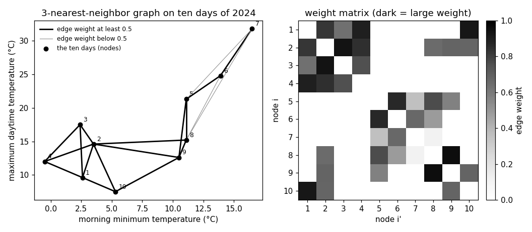
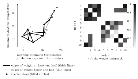
weightedgraph.py, which recomputes what the entry states: the script block by block · open in ColabB-dataConsider ten days of the year $2024$ at Krems an der Donau, every $37$th day from 1 January to 29 November, each a data point with a feature vector ${\mathbf x} \in \mathbb{R}^{2}$ that holds the morning minimum and the maximum daytime temperature of the day. Two days are similar when their feature vectors are close. A drawing records the similarities: each day is a dot, called a node, two similar days are joined by a line, called an edge, and a number on the edge says how similar the two days are. Fig. 2(a) shows this drawing for the ten days, with an edge between two days whenever one of them is among the three days nearest to the other and a number between $0$ and $1$ that falls off with the Euclidean distance between them. Nodes, edges, and a number on every edge make a weighted graph (Luxburg, 2007, Sect. 2.1; Newman, 2010).
B-weightsFormally, a weighted graph $\mathcal{G} = \left( \mathcal{V},\mathcal{E} \right)$
consists of a finite set of nodes $\mathcal{V} = \{1, \ldots,
n\}$, a set $\mathcal{E}$ of edges, and an edge weight
for each edge. Each edge is an unordered pair
$\{i,i'\}$ of two distinct nodes, so the graph
is an undirected graph without self-loops, and the two nodes
of an edge are neighbors of each other. The weight of an
edge $\{i,i'\} \in \mathcal{E}$ is a positive number
$A_{i,i'} > 0$, and a pair of nodes that
is not an edge has weight $A_{i,i'} = 0$
(Chung, 1997, Sect. 1.4). With this convention,
the weights determine the edge set, and they are collected in the
weight matrix
\begin{equation}
\label{equ_weightedgraph_weightmtx_dict}
{\mathbf A} \in \mathbb{R}^{n \times n}
\text{ with entries }
A_{i,i'} = A_{i',i}
\geq 0 \text{ and } A_{i,i} = 0
\text{ for } i, i' \in \mathcal{V} \text{.}
\end{equation}
The weight matrix \(\eqref{equ_weightedgraph_weightmtx_dict}\) is a
symmetric matrix with a zero diagonal. It is the
adjacency matrix of the graph: the entry in row $i$
and column $i'$ is the weight of the edge between
$i$ and $i'$, or zero when there is no edge
(Hastie et al., 2009, Sect. 14.5.3;
Luxburg, 2007, Sect. 2.1). An unweighted graph is the
special case in which every edge has weight $1$, so the entries of
its weight matrix \(\eqref{equ_weightedgraph_weightmtx_dict}\) are
$0$ and $1$ (Chung, 1997, Sect. 1.4).
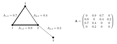
Fig. 1 shows a weighted graph with
four nodes beside its weight matrix.
What a weight means is fixed by the application, and two conventions are in use. In a road network, the nodes are intersections, the edges are road segments, and the weight of an edge is the length of the segment or the time needed to travel it (Newman, 2010). A large weight then means far apart, and the shortest route between two intersections is the path whose weights add up to the smallest value. In machine learning (ML), the weight of an edge usually measures similarity: a large weight means close together. A method that reads a similarity as a length, or a length as a similarity, inverts every conclusion it draws, so the convention must be stated. The graph in Fig. 2(a) uses the similarity convention.
B-yearThe main use of a weighted graph in ML is the
similarity graph of a dataset $\mathcal{D} = \{{\mathbf x}^{(1)},
\ldots, {\mathbf x}^{(m)}\}$. Its nodes are the
data points, $\mathcal{V} = \{1, \ldots, m\}$ with node
$r$ standing for ${\mathbf x}^{(r)}$, and the
weight of an edge measures the similarity of its two
data points. For feature vectors in $\mathbb{R}^{d}$,
a common choice is the Gaussian weight
\begin{equation}
\label{equ_weightedgraph_gauss_dict}
A_{r,r'} = \exp \Big( -
\left\lVert {\mathbf x}^{(r)} -
{\mathbf x}^{(r')} \right\rVert_{2}^{2} \big/ (2 \sigma^{2}) \Big)
\text{,}
\end{equation}
which is $1$ for two identical feature vectors and falls off
with their Euclidean distance at a rate set by the width
$\sigma > 0$ (Hastie et al., 2009, Sect. 14.5.3;
Luxburg, 2007, Sect. 2.2; Shalev-Shwartz and Ben-David, 2014, Sect. 22.3).
Giving the Gaussian weight \(\eqref{equ_weightedgraph_gauss_dict}\) to
every pair of data points produces a fully connected graph
with $m(m-1)/2$ edges, whose weight matrix has
no zero off the diagonal. A sparse alternative is the
$k$-nearest-neighbor graph ($k$-NN graph): an edge joins $r$ and $r'$ when
one of the two data points is among the $k$ nearest
data points of the other, it carries the Gaussian weight
\(\eqref{equ_weightedgraph_gauss_dict}\), and every other pair has
weight zero (Luxburg, 2007, Sect. 2.2). The width $\sigma$
and the number $k$ of neighbors are hyperparameters
of the construction; a usual choice for $\sigma$ is the mean
distance of a data point to its $k$-th nearest
neighbor (Luxburg, 2007, Sect. 8.1). For the ten days at
Krems and $k = 3$, this choice gives $\sigma = 8.27$ degrees, and
$19$ of the $45$ pairs of days are edges. Their weights range
from $0.11$, between 10 August and 16 September, to $0.95$,
between 16 September and 23 October, and the weighted degrees
\(\eqref{equ_weightedgraph_degree_dict}\) from $1.13$, on 10 August,
to $4.61$, on 7 February. Fig. 2(b)
shows the weight matrix.
pythondemos/weightedgraph.py
A weighted graph also enters empirical risk minimization (ERM) through a penalty term. In transfer learning and in federated learning (FL), the nodes are learning tasks, each with its own local dataset and a local hypothesis $h^{(i)}$, and the weight $A_{i,i'}$ states how similar two tasks are. Generalized total variation minimization (GTVMin) minimizes the sum of the local training errors plus the generalized total variation (GTV) \begin{equation} \label{equ_weightedgraph_gtv_dict} \sum_{\{i,i'\} \in \mathcal{E}} A_{i,i'} d^{(i,i')} \text{,} \end{equation} with $d^{(i,i')}$ a measure of the discrepancy between $h^{(i)}$ and $h^{(i')}$. The GTV \(\eqref{equ_weightedgraph_gtv_dict}\) couples the tasks: an edge with a large weight pulls the two hypotheses at its nodes together, and a zero weight leaves them independent. The network Lasso is the special case with the Euclidean distance between the local model parameters as the discrepancy (Hallac et al., 2015). Adding a penalty term is one of the three routes that regularization distinguishes, and the weighted graph is where this penalty term is specified. On a similarity graph of labeled and unlabeled data points, the penalty term \(\eqref{equ_weightedgraph_gtv_dict}\) with the squared difference $\big(h({\mathbf x}^{(r)}) - h({\mathbf x}^{(r')})\big)^{2}$ as the discrepancy is the Laplacian regularizer of semi-supervised learning (SSL) (Belkin et al., 2006, Sect. 2.2). It asks a hypothesis to take similar values on two data points joined by an edge of large weight, which is how the unlabeled data points shape the hypothesis. A graph neural network (GNN) uses the weights for a third purpose, to combine the feature vectors of the neighbors of each node into a new feature vector of the node.
See also: graph, undirected graph, edge weight, adjacency matrix, Laplacian matrix, node degree, neighbor, similarity graph, $k$-nearest-neighbor graph, graph clustering, spectral clustering, clustering, transfer learning, generalized total variation, generalized total variation minimization, semi-supervised learning, graph neural network, matrix.
@misc{dictml_weightedgraph,
  author = {Jung, Alexander},
  editor = {Olioumtsevits, Konstantina and Schnoor, Ekkehard},
  title = {weighted graph},
  howpublished = {Dictionary of Applied Machine Learning (course edition)},
  year = {2026},
  doi = {10.5281/zenodo.21569296},
  note = {ISBN 978-952-64-3013-3, CC BY 4.0, retrieved 2026-11-20},
  url = {https://dictionaryofml.org/terms/weightedgraph.html}
}