Density-based spatial clustering of applications with noise
(DBSCAN) is a clustering method for data points with
numeric feature vectors that finds clusters of any
shape and decides their number itself. Given a radius
$\varepsilon$ and a count $m^{*}$, a data point
is a core point if at least $m^{*}$ data points
lie within Euclidean distance $\varepsilon$ of it, and a cluster
is a maximal set of data points connected through core
points at most $\varepsilon$ apart. Data points that lie
within $\varepsilon$ of no core point are noise and belong to no
cluster. The clusters are the connected
components of the $\varepsilon$-neighborhood graph on the
core points, computed in a single pass, so DBSCAN iterates no
operator and minimizes no empirical risk. Unlike
$k$-means and a Gaussian mixture model (GMM), whose clusters are
convex regions and ellipsoids, DBSCAN finds elongated and
curved clusters, with the radius $\varepsilon$ and the
count $m^{*}$ as its hyperparameters.
B-dbscanAn aerial
photograph of the Wachau, with Weissenkirchen, Rossatz and
Duernstein along a bend of the Danube, is cut into square
patches of $76$ m, and the $1000$ patches that lie mostly on
vineyard parcels are data points, each characterized by a
feature vector ${\mathbf x} \in \mathbb{R}^{2}$ that holds its
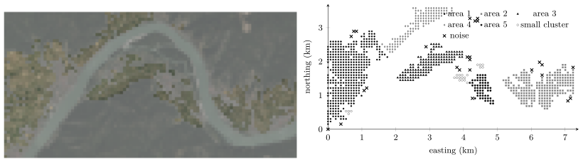
position: easting and northing in km (Fig. 1). The wine-growing areas that these
patches form follow the river banks and the slopes. They are
therefore elongated and curved, and their number is not known
in advance. DBSCAN is a clustering method for
data points with numeric feature vectors that finds
clusters of any shape and decides their number itself: a
cluster is a region in which data points lie densely,
and data points that lie in no dense region are noise
(Ester et al., 1996; Han et al., 2011). DBSCAN clusters
by density, not by shape, and
leaves isolated data points as noise. It is a
hard clustering method in the sense that every
data point belongs to at most one cluster, but unlike
a partition of the dataset it leaves the noise points
outside every cluster.
Figure 1: Top: the aerial photograph of the Wachau at patch
resolution ($7.31 \times 3.65$ km, $96 \times 48$ patches of
$76$ m); the $1000$ patches that lie mostly on vineyard
parcels keep their color, all others are dimmed. Bottom: the
same patches as data points, each drawn at its position
and marked by the cluster that DBSCAN with
$\varepsilon = 1.5$ patch spacings and $m^{*} = 4$
assigns it to: five wine-growing areas, three small
clusters, and $26$ noise patches. Orthophoto:
basemap.at (CC BY 4.0); parcels: INVEKOS 2025, AgrarMarkt
Austria (CC BY 3.0 AT). Data generated by
pythondemos/dbscan.py
DBSCAN has two hyperparameters: a radius $\varepsilon > 0$
and a count $m^{*}$. The $\varepsilon$-neighborhood of
a data point is the set of data points within
Euclidean distance $\varepsilon$ of it, the data point itself included. A data point is a core point if its
$\varepsilon$-neighborhood holds at least $m^{*}$
data points. It is a border point if it is not a core
point but lies in the $\varepsilon$-neighborhood of one, and it
is noise otherwise (Fig. 2). A
cluster is a maximal set of data points that are
connected through core points: two core points at most
$\varepsilon$ apart belong to the same cluster, and a
border point belongs to the cluster of a core point in its
$\varepsilon$-neighborhood (Ester et al., 1996). The clusters
are therefore the connected components of the
$\varepsilon$-neighborhood graph on the core points, the
graph whose edges connect core points at most
$\varepsilon$ apart, with the border points attached. DBSCAN is
a graph-based method.
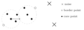
Figure 2: Core points, border points and noise for
$m^{*} = 4$. The two dashed circles are the
$\varepsilon$-neighborhoods of two core points; each holds
at least four data points. The two border points lie
within $\varepsilon$ of a core point but have fewer than
four data points in their own neighborhoods, and the
two noise points lie within $\varepsilon$ of no core point.
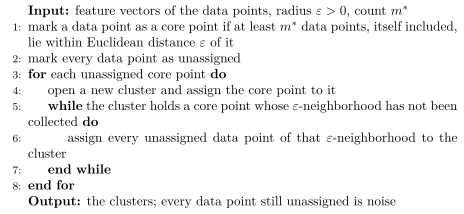
All filled and open points form one cluster DBSCAN computes the clusters in a single pass over the
data points. It picks a core point not yet assigned to a
cluster, collects every data point reachable from it
through core points at most $\varepsilon$ apart, declares the
collection a cluster, and moves on to the next core point
not yet assigned. Algorithm 1 states the
pass in full.
Algorithm 1: DBSCAN (Ester et al., 1996)
No operator is iterated, so the fixed-point iteration view
that applies to Lloyd's algorithm and the expectation–maximization (EM)
algorithm does not apply here. A second pass over the
result changes nothing, and the result depends on no
initialization, so DBSCAN has no local optima to get trapped
in. DBSCAN minimizes no empirical risk; it is defined by its
notion of a cluster alone.
On the vineyard patches with $\varepsilon = 1.5$ patch spacings
and $m^{*} = 4$, DBSCAN finds $934$ core points, $40$
border points and $26$ noise patches, grouped into eight
clusters, five of which hold at least $20$ patches: the
wine-growing areas of the strip (Fig. 1).
The river, wider than $\varepsilon$, separates the areas on its
two banks.
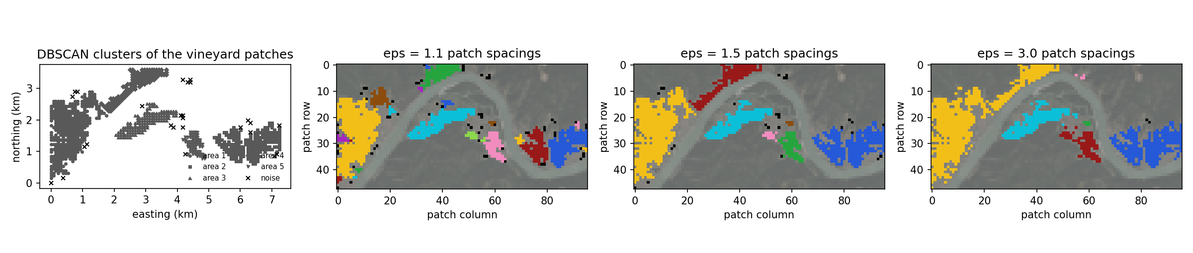
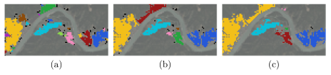
B-kmeansThe radius $\varepsilon$ decides which structures count as
clusters (Fig. 3). With
$\varepsilon = 1.1$ patch spacings, so that only the four
axis-aligned neighbors of a patch are within reach, the
patches fall into $24$ clusters with $6\%$ noise, and
several areas break along their thin stretches. With $\varepsilon = 3$ patch spacings, six clusters remain and
no patch is noise. However, two areas that $\varepsilon = 1.5$
keeps apart are joined. The number of clusters and the
noise share both fall as $\varepsilon$ grows. A common way to
choose $\varepsilon$ is to place it where the sorted
Euclidean distances of the data points to their
$m^{*}$-th nearest neighbor start to rise
steeply (Ester et al., 1996).
Figure 3: The vineyard patches of Fig. 1
painted by cluster for $m^{*} = 4$ and
(a) $\varepsilon = 1.1$, (b) $\varepsilon = 1.5$, and
(c) $\varepsilon = 3$ patch spacings; noise patches are
black. A color identifies a cluster within one
panel only, and the colors differ in brightness, so the
clusters stay apart in a grayscale print.
Orthophoto: basemap.at (CC BY 4.0). Data
generated by pythondemos/dbscan.py
DBSCAN differs from $k$-means and from a Gaussian mixture model (GMM) in three
ways. First, a cluster of $k$-means is a convex
region of the feature space and a cluster of a
GMM is an ellipsoid, whereas a DBSCAN cluster can
have any shape that a chain of nearby data points can
trace. On the vineyard patches, $k$-means with five
clusters splits one area and one of its clusters
joins two areas, since an area that curves along the river is
not convex. Second, the number of clusters is an
input of $k$-means and of a GMM but an output of
DBSCAN, at the price of the two hyperparameters
$\varepsilon$ and $m^{*}$. Third, $k$-means and a
GMM assign every data point to a cluster,
whereas DBSCAN leaves outliers as noise. DBSCAN shares
its graph-based view of a cluster with
spectral clustering. That method builds a similarity graph, a
graph whose edges connect similar data points, and
clusters its nodes by the eigenvectors of the
Laplacian matrix, a matrix that encodes the graph,
instead of by the connected components of the
$\varepsilon$-neighborhood graph.
Ester et al. (1996). A Density-Based Algorithm for Discovering Clusters in Large Spatial Databases with Noise. Proceedings of the Second International Conference on Knowledge Discovery and Data Mining.
Han et al. (2011). Data Mining: Concepts and Techniques. Morgan Kaufmann.
Cite this entry
@misc{dictml_dbscan,
  author = {Jung, Alexander},
  editor = {Olioumtsevits, Konstantina and Schnoor, Ekkehard},
  title = {density-based spatial clustering of applications with noise (DBSCAN)},
  howpublished = {Dictionary of Applied Machine Learning (course edition)},
  year = {2026},
  doi = {10.5281/zenodo.21569296},
  note = {ISBN 978-952-64-3013-3, CC BY 4.0, retrieved 2026-11-20},
  url = {https://dictionaryofml.org/terms/dbscan.html}
}