highdimregime.py, which recomputes what the entry states: the script block by block · open in ColabDictionary of Applied Machine Learning: 147 machine-learning terms, each with a definition, a figure, citations and a Python demo · All terms · Demos · Start here
Updated on 2026-11-19
Readiness 95/100
See also effective dimension overfitting generalization regularization dimensionality reduction ridge regression
A machine learning (ML) method operates in the high-dimensional regime when the effective dimension of its hypothesis space exceeds the sample size $m$ of the training set. For a linear model, the regime begins where the number $d$ of features passes the number $m$ of data points. The feature matrix then has rank at most $m$, so the least squares solution is not unique and every solution interpolates the training set. A training error of zero therefore carries no information about the risk, so the regime removes the usual evidence about generalization. Regularization and dimensionality reduction restore a usable method, the first by adding a penalty term to the training error and the second by shrinking the hypothesis space. High-dimensional statistics develops theory and methods for this regime, and its guarantees need a structural assumption such as sparsity.
highdimregime.py, which recomputes what the entry states: the script block by block · open in ColabB-leastsqConsider a weather
service at Krems an der Donau (Austria) that predicts the
maximum daytime temperature of a day from the maxima of the
previous $d$ days. Each day is a
data point with feature vector ${\mathbf x} \in
\mathbb{R}^{d}$ and label $y \in \mathbb{R}$,
and a linear model $h({\mathbf x}) =
{\mathbf w}^{\top} {\mathbf x}$ is learned by least squares
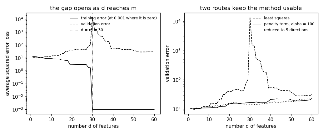
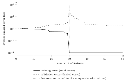
on a training set $\mathcal{D}^{(\rm train)}$ of $m = 30$ days of
$2023$. For $d = 1$, the training error is $12.4$ and
the validation error on the validation set $\mathcal{D}^{(\rm val)}$ of the $366$ days
of $2024$ is $10.1$ squared degrees. For $d = 29$, the
two numbers are $1.7$ and $100.4$, and for $d = 30$
they are $0$ and $13444$.
Once the number of features reaches the number of
data points in $\mathcal{D}^{(\rm train)}$, the training error carries no
information about the loss on days outside $\mathcal{D}^{(\rm train)}$.
Fig. 1 draws both errors for
every $d$ from $1$ to $60$.
pythondemos/highdimregime.py
B-interpThe rank of ${\mathbf X}$ is at most $m$, so for $d > m$ the nullspace of ${\mathbf X}$ holds a nonzero vector and the solution of the least squares problem \(\eqref{equ_highdimregime_leastsquares_dict}\) is not unique: its minimizers form an affine set of dimension at least $d - m$. The pseudoinverse picks the one of smallest Euclidean norm, $\widehat{{\mathbf w}} = {{\mathbf X}}^{+} {\mathbf y}$. Every minimizer drives the training error to zero, which is interpolation of $\mathcal{D}^{(\rm train)}$. The curse of dimensionality is a separate consequence of a large $d$: the data points spread thin over the feature space $\mathbb{R}^{d}$ however many of them there are, while the high-dimensional regime compares two counts.
Generalization is the performance of a learned hypothesis on data points outside $\mathcal{D}^{(\rm train)}$, and the regime removes the evidence that a small training error usually provides about it. A hypothesis that interpolates $\mathcal{D}^{(\rm train)}$ has a training error of zero whichever labels the data points of $\mathcal{D}^{(\rm train)}$ carry, so a zero training error leaves the risk undetermined and overfitting cannot be diagnosed from $\mathcal{D}^{(\rm train)}$ alone. A large artificial neural network (ANN) is trained in the same regime, with far more trainable model parameters than data points (Zhang et al., 2017, Sect. 1). A deep network reaches a training error of zero even on a training set whose labels have been replaced by random ones (Zhang et al., 2017, Sect. 2). Learning theory measures the size of $\mathcal{H}$ by its Vapnik–Chervonenkis dimension (VC dimension) and by its Rademacher complexity. The sample size that a generalization guarantee needs grows in proportion to the VC dimension (Shalev-Shwartz and Ben-David, 2014, Thm. 6.8).
B-restoreTwo routes restore a usable method on the same features,
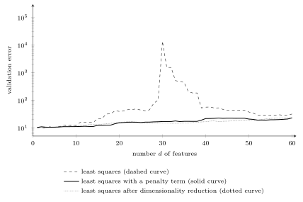
and both are forms of regularization. Adding the
penalty term $\alpha \left\lVert {\mathbf w} \right\rVert_{2}^{2}$ to
the training error gives ridge regression. With $\alpha
= 100$, the validation error of the weather example stays between
$10.2$ and $22.9$ squared degrees for every $d$ from
$1$ to $60$. Dimensionality reduction shrinks $\mathcal{H}$ instead:
least squares on the first $d' = 5$ principal
directions of the feature vectors of $\mathcal{D}^{(\rm train)}$, which is
principal component analysis (PCA), keeps the validation error between $9.8$ and $22.1$. At
$d = m$ neither learned hypothesis
interpolates $\mathcal{D}^{(\rm train)}$: the training error is $4.2$ with the
penalty term and $11.2$ after the reduction.
Fig. 2 draws the
validation error of both against the validation error of
least squares on all $d$ features.
pythondemos/highdimregime.py
See also: effective dimension, curse of dimensionality, interpolation, overfitting, generalization, regularization, dimensionality reduction, ridge regression, least absolute shrinkage and selection operator, Vapnik–Chervonenkis dimension.
@misc{dictml_highdimregime,
  author = {Jung, Alexander},
  editor = {Olioumtsevits, Konstantina and Schnoor, Ekkehard},
  title = {high-dimensional regime},
  howpublished = {Dictionary of Applied Machine Learning (course edition)},
  year = {2026},
  doi = {10.5281/zenodo.21569296},
  note = {ISBN 978-952-64-3013-3, CC BY 4.0, retrieved 2026-11-20},
  url = {https://dictionaryofml.org/terms/highdimregime.html}
}