B-restore writes when the script runsDictionary of Applied Machine Learning · high-dimensional regime
Updated on 2026-11-19
Numerical companion to the entry high-dimensional regime: it recomputes what the entry states and prints one line per check
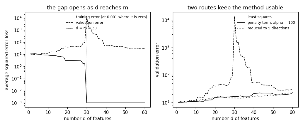
Numerical companion to the glossary entry 'highdimregime' (high-dimensional regime). A linear model predicts the maximum daytime temperature of a day at Krems (GeoSphere station 3805) from the maximum daytime temperatures of the previous d days. The training set holds m = 30 days of 2023, the validation set the 366 days of 2024. The feature count d runs from 1 to 60, so it crosses the sample size m. For d < m the hypothesis learned by least squares has a training error of the same order as its validation error. At d = m the feature matrix has rank m, the learned hypothesis interpolates the training set, the training error is zero, and the validation error is three orders of magnitude above the training error at d = 1: the training error has stopped saying anything about the loss on days outside the training set. Two routes restore a usable method on the same features, and the demo recomputes both: a penalty term (ridge regression with a fixed regularization parameter) and dimensionality reduction (least squares on the first five principal directions of the training features).
Run it without installing anything:uv run https://dictionaryofml.org/terms/highdimregime.py
uv downloads this script and the pinned NumPy and Matplotlib it needs, then runs it; the script fetches any input file it uses. To keep the output files, download highdimregime.py into a folder and run uv run highdimregime.py there. With NumPy and Matplotlib already installed, python3 highdimregime.py, from any directory — it writes its output files into the current directory. Fixed seeds, so the printed numbers reproduce exactly. Download highdimregime.py · Notebook · Open in Colab
Before running a downloaded copy, scan it: uvx bandit -q -t B102,B307,B602,B605 highdimregime.py (B102,B307,B602,B605 are the exec, eval and shell checks of bandit) reports nothing: the script runs no shell command and evaluates no generated code.
One cell per block of the script: the code, and what that code printed when it last ran here
"""The high-dimensional regime at Krems an der Donau: thirty training days
and up to sixty features, with the training error collapsing to zero and the
validation error exploding as the feature count reaches the sample size.

Purpose
-------
Numerical companion to the glossary entry 'highdimregime' (high-dimensional
regime).  A linear model predicts the maximum daytime temperature of a day
at Krems (GeoSphere station 3805) from the maximum daytime temperatures of
the previous d days.  The training set holds m = 30 days of 2023, the
validation set the 366 days of 2024.  The feature count d runs from 1 to
60, so it crosses the sample size m.  For d < m the hypothesis learned by
least squares has a training error of the same order as its validation
error.  At d = m the feature matrix has rank m, the learned hypothesis
interpolates the training set, the training error is zero, and the
validation error is three orders of magnitude above the training error at
d = 1: the training error has stopped saying anything about the loss on
days outside the training set.  Two routes restore a usable method on the
same features, and the demo recomputes both: a penalty term (ridge
regression with a fixed regularization parameter) and dimensionality
reduction (least squares on the first five principal directions of the
training features).

Self-contained (numpy and matplotlib only), fixed seeds; the GeoSphere
download falls back to the committed CSV.

Blocks
------
[B-data]     Daily maximum temperature at Krems for 2023 and 2024 (731
             days, no missing value).
[B-split]    The m = 30 training days, drawn from the 2023 days that have
             60 earlier days on record, and the 366 validation days of
             2024.
[B-leastsq]  Training and validation error of the least-squares hypothesis
             for every feature count d = 1, ..., 60.
[B-interp]   At d = m the rank of the feature matrix is m, the training
             error is zero, and the minimum-norm solution has a large
             Euclidean norm.
[B-restore]  A penalty term and dimensionality reduction keep the
             validation error below 23 squared degrees at every d.

Outputs
-------
highdimregime_weather.csv  : date, tmax for 2023 and 2024 (committed copy).
highdimregime_errors.csv   : d, training error, the same clipped at 1e-3
                             for a logarithmic axis, validation error of
                             least squares.
highdimregime_restored.csv : d, validation error of least squares, of ridge
                             regression, and after dimensionality reduction.
highdimregime.png          : matplotlib preview (checking only).
"""

# /// script
# requires-python = ">=3.10"
# dependencies = ["matplotlib==3.10.7", "numpy==2.3.4"]
# ///

import json
import urllib.request
from pathlib import Path

import numpy as np
import matplotlib

matplotlib.use("Agg")
import matplotlib.pyplot as plt

OUT_DIR = Path(__file__).parent

DMAX = 60          # largest feature count
SAMPLESIZE = 30    # m, the number of training days
REGPARAM = 100.0   # alpha, the regularization parameter of ridge regression
KEPTDIM = 5        # d', the number of kept principal directions

report = []


def check(name, ok):
    report.append((name, bool(ok)))
    print(f"  [{'ok' if ok else 'FAIL'}] {name}")
Installed 11 packages in 118ms
Daily maximum temperature at Krems for 2023 and 2024 (731 days, no missing value).
print("[B-data] daily maximum temperature at Krems, 2023 and 2024")
URL = ("https://dataset.api.hub.geosphere.at/v1/station/historical/"
       "klima-v2-1d?parameters=tlmax&station_ids=3805"
       "&start=2023-01-01&end=2024-12-31")
CSV = OUT_DIR / "highdimregime_weather.csv"
try:
    with urllib.request.urlopen(URL, timeout=120) as resp:
        payload = json.load(resp)
    params = payload["features"][0]["properties"]["parameters"]
    records = [(stamp[:10], hi)
               for stamp, hi in zip(payload["timestamps"],
                                    params["tlmax"]["data"])]
    with open(CSV, "w") as fh:
        fh.write("date,tmax\n")
        for day, hi in records:
            fh.write(f"{day},{hi}\n")
    print(f"    downloaded {len(records)} days")
except OSError as err:
    print(f"    download failed ({err}); reading the committed CSV")
    rows = CSV.read_text().strip().splitlines()[1:]
    records = [(d, float(a)) for d, a in (r.split(",") for r in rows)]

check("[B-data] 731 days for 2023 and 2024", len(records) == 731)
check("[B-data] no day is missing its maximum temperature",
      all(hi is not None for _, hi in records))
tmax = np.array([hi for _, hi in records], dtype=float)
day23 = np.array([d.startswith("2023") for d, _ in records])
check(f"[B-data] the maxima range from {tmax.min():.1f} to {tmax.max():.1f} "
      f"degrees Celsius", -20.0 < tmax.min() < tmax.max() < 45.0)
[B-data] daily maximum temperature at Krems, 2023 and 2024
    downloaded 731 days
  [ok] [B-data] 731 days for 2023 and 2024
  [ok] [B-data] no day is missing its maximum temperature
  [ok] [B-data] the maxima range from -3.6 to 35.7 degrees Celsius
The m = 30 training days, drawn from the 2023 days that have 60 earlier days on record, and the 366 validation days of 2024.
print("[B-split] the training days of 2023 and the validation days of 2024")
candidates = np.arange(DMAX, int(day23.sum()))   # 2023 days with 60 lags
rng = np.random.default_rng(2026)
train_idx = np.sort(rng.choice(candidates, size=SAMPLESIZE, replace=False))
val_idx = np.arange(int(day23.sum()), len(tmax))
check(f"[B-split] {len(train_idx)} training days of 2023, the first "
      f"{records[train_idx[0]][0]} and the last {records[train_idx[-1]][0]}",
      len(train_idx) == SAMPLESIZE and len(set(train_idx.tolist())) == SAMPLESIZE)
check(f"[B-split] {len(val_idx)} validation days, the 366 days of 2024",
      len(val_idx) == 366 and records[val_idx[0]][0] == "2024-01-01")
check("[B-split] no day belongs to both sets",
      not set(train_idx.tolist()) & set(val_idx.tolist()))
check(f"[B-split] every training day has {DMAX} earlier days on record",
      train_idx.min() >= DMAX)


def features(idx, nr_features):
    """The maxima of the nr_features days before each day in idx."""
    return np.column_stack([tmax[idx - lag]
                            for lag in range(1, nr_features + 1)])


def mean_sqerr(idx, weights, nr_features):
    residual = tmax[idx] - features(idx, nr_features) @ weights
    return float(np.mean(residual ** 2))
[B-split] the training days of 2023 and the validation days of 2024
  [ok] [B-split] 30 training days of 2023, the first 2023-03-09 and the last 2023-12-28
  [ok] [B-split] 366 validation days, the 366 days of 2024
  [ok] [B-split] no day belongs to both sets
  [ok] [B-split] every training day has 60 earlier days on record
Training and validation error of the least-squares hypothesis for every feature count d = 1, ..., 60.
print("[B-leastsq] least squares for every feature count d = 1, ..., 60")
dims = np.arange(1, DMAX + 1)
trainerr = np.empty(DMAX)
valerr = np.empty(DMAX)
solnorm = np.empty(DMAX)
ranks = np.empty(DMAX, dtype=int)
for i, d in enumerate(dims):
    Xtrain = features(train_idx, d)
    what = np.linalg.lstsq(Xtrain, tmax[train_idx], rcond=None)[0]
    trainerr[i] = mean_sqerr(train_idx, what, d)
    valerr[i] = mean_sqerr(val_idx, what, d)
    solnorm[i] = float(np.linalg.norm(what))
    ranks[i] = int(np.linalg.matrix_rank(Xtrain))

check(f"[B-leastsq] d = 1 (yesterday alone): training error "
      f"{trainerr[0]:.2f}, validation error {valerr[0]:.2f} squared degrees",
      abs(trainerr[0] - valerr[0]) < 3.0)
check(f"[B-leastsq] the training error decreases with d, from "
      f"{trainerr[0]:.2f} at d = 1 to {trainerr[SAMPLESIZE - 2]:.2f} at "
      f"d = {SAMPLESIZE - 1}", np.all(np.diff(trainerr[:SAMPLESIZE]) < 1e-9))
check(f"[B-leastsq] d = {SAMPLESIZE - 1}: training error "
      f"{trainerr[SAMPLESIZE - 2]:.2f}, validation error "
      f"{valerr[SAMPLESIZE - 2]:.1f} squared degrees",
      valerr[SAMPLESIZE - 2] > 20 * trainerr[SAMPLESIZE - 2])
check(f"[B-leastsq] the validation error is smallest at d = "
      f"{dims[valerr.argmin()]} with {valerr.min():.2f} squared degrees",
      dims[valerr.argmin()] < SAMPLESIZE)
check(f"[B-leastsq] the validation error is largest at d = "
      f"{dims[valerr.argmax()]} with {valerr.max():.0f} squared degrees",
      dims[valerr.argmax()] == SAMPLESIZE)
[B-leastsq] least squares for every feature count d = 1, ..., 60
  [ok] [B-leastsq] d = 1 (yesterday alone): training error 12.38, validation error 10.13 squared degrees
  [ok] [B-leastsq] the training error decreases with d, from 12.38 at d = 1 to 1.68 at d = 29
  [ok] [B-leastsq] d = 29: training error 1.68, validation error 100.4 squared degrees
  [ok] [B-leastsq] the validation error is smallest at d = 3 with 9.78 squared degrees
  [ok] [B-leastsq] the validation error is largest at d = 30 with 13444 squared degrees
At d = m the rank of the feature matrix is m, the training error is zero, and the minimum-norm solution has a large Euclidean norm.
print("[B-interp] interpolation of the training set at d = m")
at_m = SAMPLESIZE - 1
check(f"[B-interp] the rank of the feature matrix is min(d, m): "
      f"{ranks[0]} at d = 1, {ranks[at_m]} at d = {SAMPLESIZE}, "
      f"{ranks[-1]} at d = {DMAX}",
      np.all(ranks == np.minimum(dims, SAMPLESIZE)))
check(f"[B-interp] at d = m = {SAMPLESIZE} the training error is "
      f"{trainerr[at_m]:.2e}, zero up to rounding, so the learned "
      f"hypothesis interpolates the training set", trainerr[at_m] < 1e-20)
check(f"[B-interp] every d from {SAMPLESIZE} to {DMAX} interpolates the "
      f"training set", np.all(trainerr[at_m:] < 1e-18))
check(f"[B-interp] at d = m the validation error is {valerr[at_m]:.0f} "
      f"squared degrees, {valerr[at_m] / valerr[0]:.0f} times the "
      f"validation error {valerr[0]:.2f} at d = 1",
      valerr[at_m] > 1000 * valerr[0])
check(f"[B-interp] the minimum-norm solution grows from "
      f"{solnorm[0]:.2f} at d = 1 to {solnorm[at_m]:.1f} at d = m",
      solnorm[at_m] > 10 * solnorm[0])
[B-interp] interpolation of the training set at d = m
  [ok] [B-interp] the rank of the feature matrix is min(d, m): 1 at d = 1, 30 at d = 30, 30 at d = 60
  [ok] [B-interp] at d = m = 30 the training error is 5.86e-26, zero up to rounding, so the learned hypothesis interpolates the training set
  [ok] [B-interp] every d from 30 to 60 interpolates the training set
  [ok] [B-interp] at d = m the validation error is 13444 squared degrees, 1327 times the validation error 10.13 at d = 1
  [ok] [B-interp] the minimum-norm solution grows from 0.97 at d = 1 to 52.3 at d = m
A penalty term and dimensionality reduction keep the validation error below 23 squared degrees at every d.
print("[B-restore] a penalty term and dimensionality reduction")
ridgeerr = np.empty(DMAX)
pcaerr = np.empty(DMAX)
for i, d in enumerate(dims):
    Xtrain = features(train_idx, d)
    ytrain = tmax[train_idx]
    ridge = np.linalg.solve(Xtrain.T @ Xtrain + REGPARAM * np.eye(d),
                            Xtrain.T @ ytrain)
    ridgeerr[i] = mean_sqerr(val_idx, ridge, d)
    kept = min(KEPTDIM, d)
    basis = np.linalg.svd(Xtrain, full_matrices=False)[2][:kept].T
    coeff = np.linalg.lstsq(Xtrain @ basis, ytrain, rcond=None)[0]
    pcaerr[i] = mean_sqerr(val_idx, basis @ coeff, d)

check(f"[B-restore] ridge regression with alpha = {REGPARAM:.0f} keeps the "
      f"validation error between {ridgeerr.min():.1f} and "
      f"{ridgeerr.max():.1f} squared degrees over all 60 feature counts",
      ridgeerr.max() < 23.0)
check(f"[B-restore] least squares on the first {KEPTDIM} principal "
      f"directions keeps it between {pcaerr.min():.1f} and "
      f"{pcaerr.max():.1f}", pcaerr.max() < 23.0)
check(f"[B-restore] at d = m both stay near their value at d = 1: ridge "
      f"{ridgeerr[at_m]:.1f} against {ridgeerr[0]:.1f}, reduced "
      f"{pcaerr[at_m]:.1f} against {pcaerr[0]:.1f}",
      ridgeerr[at_m] < 3 * ridgeerr[0] and pcaerr[at_m] < 3 * pcaerr[0])
check(f"[B-restore] at d = m both are below the least-squares validation "
      f"error {valerr[at_m]:.0f} by a factor above 500",
      valerr[at_m] / max(ridgeerr[at_m], pcaerr[at_m]) > 500.0)
Xm = features(train_idx, SAMPLESIZE)
ridge_m = np.linalg.solve(Xm.T @ Xm + REGPARAM * np.eye(SAMPLESIZE),
                          Xm.T @ tmax[train_idx])
basis_m = np.linalg.svd(Xm, full_matrices=False)[2][:KEPTDIM].T
coeff_m = np.linalg.lstsq(Xm @ basis_m, tmax[train_idx], rcond=None)[0]
check(f"[B-restore] at d = m neither route interpolates the training set: "
      f"training error {mean_sqerr(train_idx, ridge_m, SAMPLESIZE):.2f} with "
      f"the penalty term and "
      f"{mean_sqerr(train_idx, basis_m @ coeff_m, SAMPLESIZE):.2f} after the "
      f"reduction, against {trainerr[at_m]:.2e} for least squares",
      min(mean_sqerr(train_idx, ridge_m, SAMPLESIZE),
          mean_sqerr(train_idx, basis_m @ coeff_m, SAMPLESIZE)) > 1.0)


# ---- CSVs and preview
FLOOR = 1e-3   # a log axis cannot draw a zero training error
with open(OUT_DIR / "highdimregime_errors.csv", "w") as fh:
    fh.write("d,trainerr,trainplot,valerr\n")
    for i, d in enumerate(dims):
        fh.write(f"{d},{trainerr[i]:.6g},{max(trainerr[i], FLOOR):.6g},"
                 f"{valerr[i]:.6g}\n")
with open(OUT_DIR / "highdimregime_restored.csv", "w") as fh:
    fh.write("d,leastsquares,ridge,reduced\n")
    for i, d in enumerate(dims):
        fh.write(f"{d},{valerr[i]:.6g},{ridgeerr[i]:.6g},{pcaerr[i]:.6g}\n")

fig, (ax1, ax2) = plt.subplots(1, 2, figsize=(9.4, 3.9))
ax1.semilogy(dims, np.maximum(trainerr, FLOOR), "k-", lw=1.1,
             label=f"training error (at {FLOOR:g} where it is zero)")
ax1.semilogy(dims, valerr, "k--", lw=1.1, label="validation error")
ax1.axvline(SAMPLESIZE, color="black", ls=":", lw=0.9,
            label=f"d = m = {SAMPLESIZE}")
ax1.set_xlabel("number d of features")
ax1.set_ylabel("average squared error loss")
ax1.set_title("the gap opens as d reaches m")
ax1.legend(frameon=False, fontsize=8)
ax2.semilogy(dims, valerr, "k--", lw=1.1, label="least squares")
ax2.semilogy(dims, ridgeerr, "k-", lw=1.1,
             label=f"penalty term, alpha = {REGPARAM:.0f}")
ax2.semilogy(dims, pcaerr, "k:", lw=1.3,
             label=f"reduced to {KEPTDIM} directions")
ax2.set_xlabel("number d of features")
ax2.set_ylabel("validation error")
ax2.set_title("two routes keep the method usable")
ax2.legend(frameon=False, fontsize=8)
fig.tight_layout()
fig.savefig(OUT_DIR / "highdimregime.png", dpi=110)

n_ok = sum(ok for _, ok in report)
print(f"\n{n_ok}/{len(report)} checks pass")
if n_ok != len(report):
    raise SystemExit(1)
[B-restore] a penalty term and dimensionality reduction
  [ok] [B-restore] ridge regression with alpha = 100 keeps the validation error between 10.2 and 22.9 squared degrees over all 60 feature counts
  [ok] [B-restore] least squares on the first 5 principal directions keeps it between 9.8 and 22.1
  [ok] [B-restore] at d = m both stay near their value at d = 1: ridge 16.8 against 10.2, reduced 14.7 against 10.1
  [ok] [B-restore] at d = m both are below the least-squares validation error 13444 by a factor above 500
  [ok] [B-restore] at d = m neither route interpolates the training set: training error 4.24 with the penalty term and 11.19 after the reduction, against 5.86e-26 for least squares

22/22 checks pass
B-restore writes when the script runs