effdim.py, which recomputes what the entry states: the script block by block · open in ColabDictionary of Applied Machine Learning: 111 machine-learning terms, each with a definition, a figure, citations and a Python demo · All terms · Demos · Start here
Updated on 2026-10-29
Readiness 75/100
See also hypothesis space feature matrix probability distribution generalization
The effective dimension of a hypothesis space is its size as seen through the probability distribution of the features: the number of model parameters that make a difference on the data points the distribution produces. For a linear model it is the rank of the second-moment matrix of the feature map, estimated by the rank of the feature matrix, and it never exceeds the number of model parameters. Two hypothesis spaces that differ only outside the support of the distribution have the same effective dimension, and empirical risk minimization (ERM) on them delivers the same predictions on the data. The same hypothesis space can have different effective dimensions under different data distributions. The Rademacher complexity is the distribution-dependent size measure of learning theory, while the Vapnik–Chervonenkis dimension (VC dimension) is its worst case over the whole feature space.
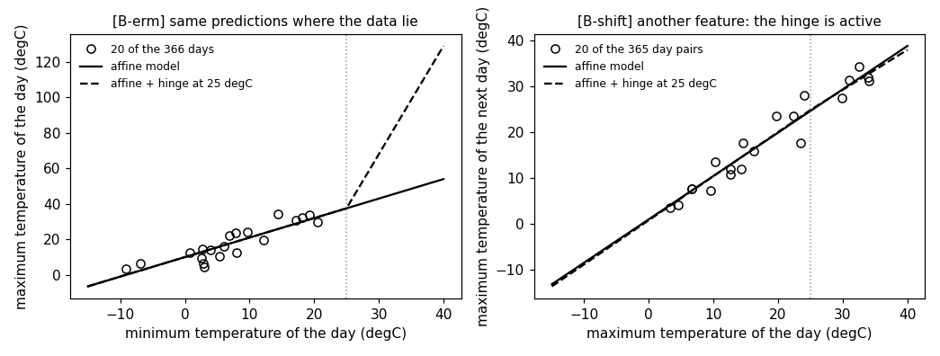
effdim.py, which recomputes what the entry states: the script block by block · open in ColabB-dataConsider the $366$ days of $2024$ at the weather station Krems an der Donau, each a data point with the minimum temperature of the day as its feature $x$ and the maximum temperature as its label $y$. Two hypothesis spaces are candidates for predicting $y$ from $x$: the affine linear model $\mathcal{H}^{(1)} = \{ w_{0} + w_{1} x \}$ with two model parameters, and the linear model $\mathcal{H}^{(2)} = \{ w_{0} + w_{1} x + w_{2} \max(0, x - 25) \}$ with three, whose third feature is a rectified linear unit (ReLU) hinge at $25\,^{\circ}$C. The minimum temperature of the record ranges from $-10.1$ to $20.8\,^{\circ}$C, so the hinge is zero on every day. On this record, every hypothesis of $\mathcal{H}^{(2)}$ agrees with a hypothesis of $\mathcal{H}^{(1)}$: the third model parameter changes no prediction that the data can test.
B-rankThe effective dimension $d_{\rm eff} \left( \mathcal{H} \right)$ of a hypothesis space $\mathcal{H}$ is its size as seen through the probability distribution $\mathbb{P}^{(x)}$ of the features: it counts the model parameters that make a difference on the data points the distribution produces, not the model parameters that are written down. For a linear model with feature map ${\mathbf \Phi}$, the effective dimension is the rank of the second-moment matrix $\mathbb{E}\big\{ {\mathbf \Phi}(x) {\mathbf \Phi}(x)^{\top} \big\}$, which a dataset estimates by the rank of its feature matrix (Hastie et al., 2009, Sect. 7.6). It never exceeds the number of model parameters, and it equals that number only when the features are linearly independent on the support of $\mathbb{P}^{(x)}$. On the Krems record the feature matrix of $\mathcal{H}^{(2)}$ has three columns and rank $2$, since its hinge column is zero, so $d_{\rm eff} \left( \mathcal{H}^{(1)} \right) = d_{\rm eff} \left( \mathcal{H}^{(2)} \right) = 2$. Two hypothesis spaces that differ only outside the support of $\mathbb{P}^{(x)}$ have the same effective dimension.
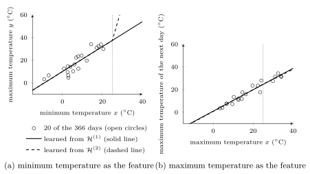
B-ermThe consequence for empirical risk minimization (ERM) is visible in Fig. 1(a). Least squares on $\mathcal{H}^{(1)}$ and on $\mathcal{H}^{(2)}$ delivers the same prediction for every day of the record and the same training error of $19.2$ squared degrees. The hinge coefficient $w_{2}$ is not identifiable: every value gives the same training error, and the two learned hypotheses differ only for a minimum temperature above $25\,^{\circ}$C, a region that no day of the record reaches. There the data say nothing, which is the generalization problem in its sharpest form: a hypothesis is tested only where the features lie.
B-shiftThe effective dimension depends on the probability distribution, not only on
the hypothesis space. Fig. 1(b) keeps
$\mathcal{H}^{(2)}$ and changes the feature to the maximum
temperature of the day, with the maximum temperature of the next
day as the label. The maximum temperature exceeds
$25\,^{\circ}$C on $97$ of the $365$ day pairs, the hinge column of
the feature matrix is no longer zero, its rank is $3$, and
least squares on $\mathcal{H}^{(2)}$ now reaches a smaller
training error than on $\mathcal{H}^{(1)}$, if only slightly. The same
hypothesis space has effective dimension $2$ under one data
distribution and $3$ under another.
pythondemos/effdim.py
See also: hypothesis space, model parameter, dimension, linear model, feature map, feature matrix, rank, probability distribution, generalization, Vapnik–Chervonenkis dimension, Rademacher complexity, ridge regression.
@misc{dictml_effdim,
  author = {Jung, Alexander},
  editor = {Olioumtsevits, Konstantina and Schnoor, Ekkehard},
  title = {effective dimension},
  howpublished = {Dictionary of Applied Machine Learning (course edition)},
  year = {2026},
  doi = {10.5281/zenodo.21569296},
  note = {ISBN 978-952-64-3013-3, CC BY 4.0, retrieved 2026-10-29},
  url = {https://dictionaryofml.org/terms/effdim.html}
}