B-shift writes when the script runsDictionary of Applied Machine Learning · effective dimension
Numerical companion to the entry effective dimension: it recomputes what the entry states and prints one line per check
The entry's point: the effective dimension of a hypothesis space is a property of the pair (hypothesis space, probability distribution of the data), not of the hypothesis space alone. Two hypothesis spaces that differ only where the data never lie have the same effective dimension, and one hypothesis space has different effective dimensions under two distributions. The demo uses the 366 days of 2024 at Krems an der Donau (GeoSphere Austria archive), feature = minimum temperature of the day, label = maximum temperature of the day, and a linear model with the feature map phi(x) = (1, x, max(0, x - 25)): the third feature, a hinge at 25 degC, is zero for every day of the record, since the minimum temperature never reaches 25 degC. Self-contained (numpy/matplotlib only), no randomness beyond the fixed-seed choice of plotted days.
Run it without installing anything:uv run https://dictionaryofml.org/terms/effdim.py
uv downloads this script and the pinned NumPy and Matplotlib it needs, then runs it; the script fetches any input file it uses. To keep the output files, download effdim.py into a folder and run uv run effdim.py there. With NumPy and Matplotlib already installed, python3 effdim.py, from any directory — it writes its output files into the current directory. Fixed seeds, so the printed numbers reproduce exactly. Download effdim.py · Notebook · Open in Colab
One cell per block of the script: the code, and what that code printed when it last ran here
"""
effdim.py — numerical companion to the glossary entry 'effdim'
(effective dimension).

The entry's point: the effective dimension of a hypothesis space is a
property of the pair (hypothesis space, probability distribution of the
data), not of the hypothesis space alone. Two hypothesis spaces that
differ only where the data never lie have the same effective dimension,
and one hypothesis space has different effective dimensions under two
distributions. The demo uses the 366 days of 2024 at Krems an der Donau
(GeoSphere Austria archive), feature = minimum temperature of the day,
label = maximum temperature of the day, and a linear model with the
feature map phi(x) = (1, x, max(0, x - 25)): the third feature, a hinge
at 25 degC, is zero for every day of the record, since the minimum
temperature never reaches 25 degC. Self-contained (numpy/matplotlib
only), no randomness beyond the fixed-seed choice of plotted days.

Blocks
------
[B-data]  The 366 days; the minimum temperature ranges over
          [-10.1, 20.8] degC, so the hinge feature max(0, x - 25) is
          identically zero on the record.
[B-rank]  The feature matrix of phi over the record has rank 2, not 3:
          the effective dimension of the hinge model relative to this
          data distribution is 2, the same as that of the affine model
          (1, x). The sample second-moment matrix of phi has the same
          rank.
[B-erm]   Least squares on both models delivers the same predictions on
          every day of the record and the same training error; the
          hinge coefficient is not identifiable (the minimum-norm
          solution sets it to 0, any other value gives the same
          training error). Outside the record's range, i.e., for x > 25,
          the two learned hypotheses differ.
[B-shift] Under another data distribution the ranks differ: with the
          maximum temperature of the day as the feature (range
          [-3.6, 34.3] degC), the hinge is active on the hot days, the
          feature matrix has rank 3, and least squares on the hinge
          model reaches a smaller training error than the affine model
          when predicting the next day's maximum.

Outputs
-------
effdim_points_plot.csv : 20 of the 366 days (every 19th in date order),
                         tmin, tmax.
effdim_lines.csv       : the two learned hypotheses of [B-erm] on a grid
                         over [-15, 40] degC, columns x, affine, hinge.
effdim_shift_plot.csv  : 20 of the 365 day pairs of [B-shift] (every
                         19th), tmax_today, tmax_next.
effdim_shift_lines.csv : the two learned hypotheses of [B-shift] on the
                         same grid, columns x, affine, hinge.
effdim.png             : preview figure (checking only).

Data generated by pythondemos/effdim.py.
"""

import json
import urllib.request
import numpy as np
import matplotlib

matplotlib.use("Agg")
import matplotlib.pyplot as plt
from pathlib import Path

OUT_DIR = Path(__file__).parent
ARCHIVE = "https://dataset.api.hub.geosphere.at/v1/station/historical/"
STATION = 3805                      # Krems an der Donau
KNOT = 25.0                         # the hinge sits at 25 degC
EVERY = 19                          # every 19th day is plotted: 20 of 366
GRID = np.linspace(-15.0, 40.0, 221)
report = []


def check(name, ok):
    report.append((name, bool(ok)))
    print(f"  [{'ok' if ok else 'FAIL'}] {name}")


def fetch(parameters, start, end):
    """Daily parameters of one station from the GeoSphere Austria archive."""
    url = (f"{ARCHIVE}klima-v2-1d?parameters={','.join(parameters)}"
           f"&station_ids={STATION}&start={start}&end={end}")
    with urllib.request.urlopen(url, timeout=180) as resp:
        payload = json.load(resp)
    values = payload["features"][0]["properties"]["parameters"]
    return np.stack([np.array(values[p]["data"], dtype=float)
                     for p in parameters], axis=1)


def phi_affine(x):
    return np.stack([np.ones_like(x), x], axis=1)


def phi_hinge(x):
    return np.stack([np.ones_like(x), x, np.maximum(0.0, x - KNOT)], axis=1)


def least_squares(X, y):
    """Minimum-norm least-squares weights and the average squared error."""
    w = np.linalg.lstsq(X, y, rcond=None)[0]
    return w, float(np.mean((X @ w - y) ** 2))


def write_rows(name, header, rows):
    with open(OUT_DIR / name, "w") as f:
        f.write(header + "\n")
        for r in rows:
            f.write(",".join(f"{v:.3f}" for v in r) + "\n")
The 366 days; the minimum temperature ranges over [-10.1, 20.8] degC, so the hinge feature max(0, x - 25) is identically zero on the record.
days = fetch(["tlmin", "tlmax"], "2024-01-01", "2024-12-31")
tmin, tmax = days[:, 0], days[:, 1]
m = tmin.size
print(f"[B-data] {m} days at Krems an der Donau, 2024; minimum temperature "
      f"in [{tmin.min():.1f}, {tmin.max():.1f}] degC, maximum in "
      f"[{tmax.min():.1f}, {tmax.max():.1f}] degC")
check("[B-data] one full (leap) year, no gaps", m == 366 and not np.isnan(days).any())
check("[B-data] the minimum temperature never reaches the hinge at 25 degC",
      tmin.max() < KNOT)
check("[B-data] so the hinge feature is identically zero on the record",
      np.all(phi_hinge(tmin)[:, 2] == 0.0))
plot_idx = np.arange(0, m, EVERY)[:20]
write_rows("effdim_points_plot.csv", "tmin,tmax",
           [(tmin[i], tmax[i]) for i in plot_idx])
check("[B-data] 20 of the 366 days are written for the plot", plot_idx.size == 20)
[B-data] 366 days at Krems an der Donau, 2024; minimum temperature in [-10.1, 20.8] degC, maximum in [-3.6, 34.3] degC
  [ok] [B-data] one full (leap) year, no gaps
  [ok] [B-data] the minimum temperature never reaches the hinge at 25 degC
  [ok] [B-data] so the hinge feature is identically zero on the record
  [ok] [B-data] 20 of the 366 days are written for the plot
The feature matrix of phi over the record has rank 2, not 3: the effective dimension of the hinge model relative to this data distribution is 2, the same as that of the affine model (1, x). The sample second-moment matrix of phi has the same rank.
X_aff, X_hin = phi_affine(tmin), phi_hinge(tmin)
r_aff, r_hin = np.linalg.matrix_rank(X_aff), np.linalg.matrix_rank(X_hin)
M_hin = X_hin.T @ X_hin / m
print(f"[B-rank] rank of the feature matrix: affine model {r_aff}, hinge "
      f"model {r_hin} (three columns); rank of the sample second-moment "
      f"matrix of the hinge map {np.linalg.matrix_rank(M_hin)}")
check("[B-rank] the affine model has effective dimension 2", r_aff == 2)
check("[B-rank] the hinge model has effective dimension 2 on this "
      "distribution too, not 3", r_hin == 2)
check("[B-rank] the sample second-moment matrix of the hinge map has rank 2",
      np.linalg.matrix_rank(M_hin) == 2)
[B-rank] rank of the feature matrix: affine model 2, hinge model 2 (three columns); rank of the sample second-moment matrix of the hinge map 2
  [ok] [B-rank] the affine model has effective dimension 2
  [ok] [B-rank] the hinge model has effective dimension 2 on this distribution too, not 3
  [ok] [B-rank] the sample second-moment matrix of the hinge map has rank 2
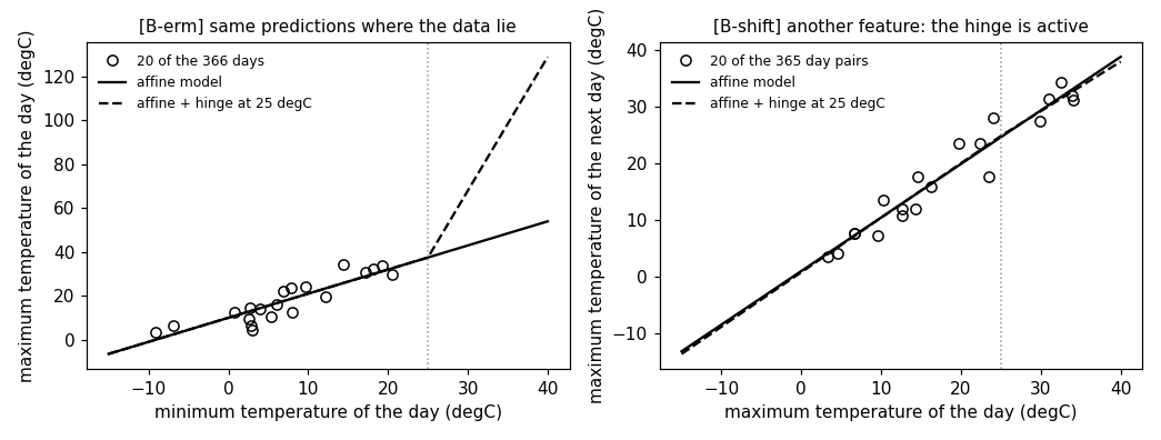
Least squares on both models delivers the same predictions on every day of the record and the same training error; the hinge coefficient is not identifiable (the minimum-norm solution sets it to 0, any other value gives the same training error). Outside the record's range, i.e., for x > 25, the two learned hypotheses differ.
w_aff, err_aff = least_squares(X_aff, tmax)
w_hin, err_hin = least_squares(X_hin, tmax)
pred_aff, pred_hin = X_aff @ w_aff, X_hin @ w_hin
print(f"[B-erm] affine: tmax = {w_aff[0]:.2f} + {w_aff[1]:.3f} tmin, training "
      f"error {err_aff:.2f}; hinge model: same two coefficients "
      f"({w_hin[0]:.2f}, {w_hin[1]:.3f}) and hinge coefficient {w_hin[2]:.3f}, "
      f"training error {err_hin:.2f}")
check("[B-erm] the two learned hypotheses agree on every day of the record",
      np.allclose(pred_aff, pred_hin))
check("[B-erm] and have the same training error", abs(err_aff - err_hin) < 1e-9)
w_other = w_hin.copy(); w_other[2] = 5.0
check("[B-erm] the hinge coefficient is not identifiable: any value gives "
      "the same training error",
      abs(np.mean((X_hin @ w_other - tmax) ** 2) - err_hin) < 1e-9)
line_hin = phi_hinge(GRID) @ w_other       # the hinge drawn with slope 5 beyond 25 degC
line_aff = phi_affine(GRID) @ w_aff
check("[B-erm] outside the record's range the two hypotheses differ",
      np.max(np.abs(line_hin[GRID > KNOT] - line_aff[GRID > KNOT])) > 10)
check("[B-erm] and on the record's range they coincide",
      np.allclose(line_hin[GRID <= KNOT], line_aff[GRID <= KNOT]))
write_rows("effdim_lines.csv", "x,affine,hinge",
           zip(GRID, line_aff, line_hin))
[B-erm] affine: tmax = 10.02 + 1.099 tmin, training error 19.17; hinge model: same two coefficients (10.02, 1.099) and hinge coefficient 0.000, training error 19.17
  [ok] [B-erm] the two learned hypotheses agree on every day of the record
  [ok] [B-erm] and have the same training error
  [ok] [B-erm] the hinge coefficient is not identifiable: any value gives the same training error
  [ok] [B-erm] outside the record's range the two hypotheses differ
  [ok] [B-erm] and on the record's range they coincide
Under another data distribution the ranks differ: with the maximum temperature of the day as the feature (range [-3.6, 34.3] degC), the hinge is active on the hot days, the feature matrix has rank 3, and least squares on the hinge model reaches a smaller training error than the affine model when predicting the next day's maximum.
x2, y2 = tmax[:-1], tmax[1:]          # today's maximum predicts tomorrow's
X2_aff, X2_hin = phi_affine(x2), phi_hinge(x2)
r2_aff, r2_hin = np.linalg.matrix_rank(X2_aff), np.linalg.matrix_rank(X2_hin)
w2_aff, err2_aff = least_squares(X2_aff, y2)
w2_hin, err2_hin = least_squares(X2_hin, y2)
hot = int(np.sum(x2 > KNOT))
print(f"[B-shift] feature = maximum temperature: {hot} of {x2.size} days "
      f"exceed 25 degC; ranks affine {r2_aff}, hinge {r2_hin}; training "
      f"errors affine {err2_aff:.2f}, hinge {err2_hin:.2f}")
check("[B-shift] the hinge is active on some days", hot > 0)
check("[B-shift] the hinge model now has effective dimension 3", r2_hin == 3)
check("[B-shift] and least squares on it reaches a smaller training error "
      "than the affine model", err2_hin < err2_aff - 1e-6)
plot2 = np.arange(0, x2.size, EVERY)[:20]
write_rows("effdim_shift_plot.csv", "tmax_today,tmax_next",
           [(x2[i], y2[i]) for i in plot2])
write_rows("effdim_shift_lines.csv", "x,affine,hinge",
           zip(GRID, phi_affine(GRID) @ w2_aff, phi_hinge(GRID) @ w2_hin))

# ------------------------------------------------------------- preview
fig, ax = plt.subplots(1, 2, figsize=(9.5, 3.6))
ax[0].plot(tmin[plot_idx], tmax[plot_idx], "o", mfc="none", color="black",
           label="20 of the 366 days")
ax[0].plot(GRID, line_aff, "k-", label="affine model")
ax[0].plot(GRID, line_hin, "k--", label="affine + hinge at 25 degC")
ax[0].axvline(KNOT, color="0.6", linestyle=":", linewidth=1)
ax[0].set_xlabel("minimum temperature of the day (degC)")
ax[0].set_ylabel("maximum temperature of the day (degC)")
ax[0].set_title("[B-erm] same predictions where the data lie", fontsize=10)
ax[0].legend(frameon=False, fontsize=8)
ax[1].plot(x2[plot2], y2[plot2], "o", mfc="none", color="black",
           label="20 of the 365 day pairs")
ax[1].plot(GRID, phi_affine(GRID) @ w2_aff, "k-", label="affine model")
ax[1].plot(GRID, phi_hinge(GRID) @ w2_hin, "k--", label="affine + hinge at 25 degC")
ax[1].axvline(KNOT, color="0.6", linestyle=":", linewidth=1)
ax[1].set_xlabel("maximum temperature of the day (degC)")
ax[1].set_ylabel("maximum temperature of the next day (degC)")
ax[1].set_title("[B-shift] another feature: the hinge is active", fontsize=10)
ax[1].legend(frameon=False, fontsize=8)
fig.tight_layout()
fig.savefig(OUT_DIR / "effdim.png", dpi=110)
print(f"\n{sum(ok for _, ok in report)}/{len(report)} checks passed")
assert all(ok for _, ok in report)
[B-shift] feature = maximum temperature: 97 of 365 days exceed 25 degC; ranks affine 2, hinge 3; training errors affine 9.83, hinge 9.81
  [ok] [B-shift] the hinge is active on some days
  [ok] [B-shift] the hinge model now has effective dimension 3
  [ok] [B-shift] and least squares on it reaches a smaller training error than the affine model

15/15 checks passed
B-shift writes when the script runs