decisionregion.py, which recomputes what the entry states: the script block by block · open in ColabDictionary of Applied Machine Learning: 115 machine-learning terms, each with a definition, a figure, citations and a Python demo · All terms · Demos · Start here
Updated on 2026-11-08
Readiness 80/100
See also classification binary classification decision boundary linear classifier decision tree logistic regression
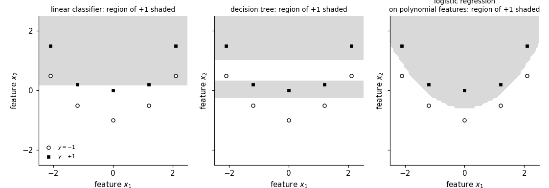
A decision region of a classifier is the set of all feature vectors that the classifier maps to one particular label value. The decision regions partition the feature space, one region per label value, and all feature vectors in the same region obtain the same prediction, so the decision regions determine the classifier completely. The union of the boundaries of the decision regions is the decision boundary. The shape of the decision regions depends on the model: a linear classifier has halfspaces, a decision tree has unions of axis-parallel rectangles, and logistic regression on polynomial features has regions separated by a curve.
decisionregion.py, which recomputes what the entry states: the script block by block · open in ColabB-partitionA frost warning predicts from the minimum and the maximum air temperature of a day whether the following night brings frost. Any rule that gives this warning splits the pairs of temperatures into two parts: the pairs for which it predicts frost and the pairs for which it does not. Each part is a decision region of the rule. In general, a classifier is a hypothesis $h\colon \mathcal{X} \rightarrow \mathcal{Y}$ with a finite label space $\mathcal{Y}$. Its decision region for the label value $\widehat{y} \in \mathcal{Y}$ is the set of feature vectors that it maps to this value, \[ \mathcal{R}_{\widehat{y}} := \big\{ {\mathbf x} \in \mathcal{X} : h({\mathbf x}) = \widehat{y} \big\} \text{.} \] The decision regions partition the feature space: every feature vector lies in exactly one of them, there is one region per label value, and a region may consist of several separate pieces (Bishop, 2006, Sect. 1.5.1). All feature vectors in the same decision region obtain the same prediction, so the decision regions determine the classifier completely. The boundary $\partial \mathcal{R}_{\widehat{y}}$ of a decision region is the set of feature vectors such that every neighborhood contains elements of $\mathcal{R}_{\widehat{y}}$ and of its complement. The union of these boundaries over all label values is the decision boundary.
B-shapeThe shape of the decision regions depends on the model. A linear classifier with $h({\mathbf x}) = \operatorname{sign}({\mathbf w}^{\top} {\mathbf x} + w_{0})$ has the two halfspaces on either side of the hyperplane ${\mathbf w}^{\top} {\mathbf x} + w_{0} = 0$ as its decision regions (Bishop, 2006, Sect. 4.1.1). For more than two label values, a linear classifier predicts the value with the largest of $K$ linear scores. Each decision region is then an intersection of $K - 1$ halfspaces and therefore convex (Bishop, 2006, Sect. 4.1.2). A decision tree compares one feature with a threshold at each split, so its decision regions are unions of axis-parallel rectangles (Hastie et al., 2009, Sect. 9.2.1). Logistic regression on polynomial features has decision regions separated by a curve, the level set of a polynomial.
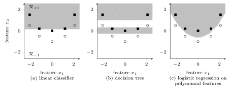
B-determinedFig. 1 shows the decision regions
of three classifiers learned from the same
data points with two features: a linear classifier, a
decision tree, and logistic regression on polynomial
features. A data point whose label differs
from the label value of the region containing its
feature vector is misclassified, and the fraction of such
data points is the average $0/1$ loss. The two
label values are separated by a curve and not by any
straight line, so the linear classifier misclassifies half of the
data points, while the other two misclassify none.
pythondemos/decisionregion.py
See also: classifier, classification, binary classification, decision boundary, boundary, neighborhood, linear classifier, decision tree, logistic regression, halfspace, hyperplane, feature space, label space, $\bf 0/1$ loss.
@misc{dictml_decisionregion,
  author = {Jung, Alexander},
  editor = {Olioumtsevits, Konstantina and Schnoor, Ekkehard},
  title = {decision region},
  howpublished = {Dictionary of Applied Machine Learning (course edition)},
  year = {2026},
  doi = {10.5281/zenodo.21569296},
  note = {ISBN 978-952-64-3013-3, CC BY 4.0, retrieved 2026-11-11},
  url = {https://dictionaryofml.org/terms/decisionregion.html}
}