B-determined writes when the script runsDictionary of Applied Machine Learning · decision region
Updated on 2026-11-06
Numerical companion to the entry decision region: it recomputes what the entry states and prints one line per check
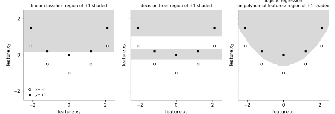
Backs the entry's claims numerically, on the training set and the three classifiers of the entry 'decision boundary' (pythondemos/ decisionboundary.py): the decision regions of a classifier partition the feature space, one region per label value; their shape depends on the model (two half-planes for a linear classifier, unions of axis-parallel rectangles for a decision tree, a region with a curved border for logistic regression on polynomial features); and the regions determine the classifier completely, so the prediction for a data point is the label value of the region its feature vector lies in, and the average zero-one loss is the fraction of data points lying in the region of the other label value. Self-contained (numpy and matplotlib only), no randomness.
Run it without installing anything:uv run https://dictionaryofml.org/terms/decisionregion.py
uv downloads this script and the pinned NumPy and Matplotlib it needs, then runs it; the script fetches any input file it uses. To keep the output files, download decisionregion.py into a folder and run uv run decisionregion.py there. With NumPy and Matplotlib already installed, python3 decisionregion.py, from any directory — it writes its output files into the current directory. Fixed seeds, so the printed numbers reproduce exactly. Download decisionregion.py · Notebook · Open in Colab
Before running a downloaded copy, scan it: uvx bandit -q -t B102,B307,B602,B605 decisionregion.py (B102,B307,B602,B605 are the exec, eval and shell checks of bandit) reports nothing: the script runs no shell command and evaluates no generated code.
One cell per block of the script: the code, and what that code printed when it last ran here
"""
decisionregion.py — numerical companion to the glossary entry 'decision
region'.

Purpose
-------
Backs the entry's claims numerically, on the training set and the three
classifiers of the entry 'decision boundary' (pythondemos/
decisionboundary.py): the decision regions of a classifier partition the
feature space, one region per label value; their shape depends on the
model (two half-planes for a linear classifier, unions of axis-parallel
rectangles for a decision tree, a region with a curved border for logistic
regression on polynomial features); and the regions determine the
classifier completely, so the prediction for a data point is the label
value of the region its feature vector lies in, and the average zero-one
loss is the fraction of data points lying in the region of the other label
value.  Self-contained (numpy and matplotlib only), no randomness.

Setup
-----
The same ten data points with two features as in decisionboundary.py, whose
label values y = +1 and y = -1 are separated by a parabola, and the same
three classifiers learned from them: logistic regression on the two
features (a linear classifier), a decision tree of depth at most four, and
logistic regression on all monomials of the two features up to degree two.
The regions are evaluated on a grid of 60 x 60 points over [-2.5, 2.5]^2.

Blocks
------
[B-partition]  For each classifier, every grid point lies in exactly one of
               its two decision regions, and both regions are nonempty.
[B-shape]      The linear classifier's region of +1 is the set of grid
               points with w^T x + w_0 >= 0, and the midpoint of two grid
               points of one region lies in that region (half-planes,
               convex); the decision tree's prediction is constant on each
               rectangle cut out by its thresholds (unions of axis-parallel
               rectangles); the lower border of the polynomial classifier's
               region of +1 is lower at x1 = 0 than at x1 = -2 and x1 = 2
               (not a straight line).
[B-determined] The label value of the region containing a data point's
               feature vector, found by the half-plane test for the linear
               classifier and by the rectangle table for the tree, is the
               classifier's prediction; for each classifier, the number of
               data points lying in the region of the other label value,
               divided by ten, is its average zero-one loss.

Outputs
-------
decisionregion_points.csv  : x1, x2, y of the ten data points.
decisionregion_regions.csv : the grid with the label predicted by the
                             linear classifier (lin), the decision tree
                             (tree) and the polynomial classifier (poly);
                             60 columns per row, rows ordered by x2.
decisionregion.png         : matplotlib preview (checking only).
"""

# /// script
# requires-python = ">=3.10"
# dependencies = ["matplotlib==3.10.7", "numpy==2.3.4"]
# ///

import numpy as np
import matplotlib

matplotlib.use("Agg")
import matplotlib.pyplot as plt

from pathlib import Path

OUT_DIR = Path(__file__).parent

report = []


def check(name, ok):
    report.append((name, bool(ok)))
    print(f"  [{'ok' if ok else 'FAIL'}] {name}")


# the ten data points of decisionboundary.py, separated by a parabola
X = np.array([
    [-2.1, 1.5], [-1.2, 0.2], [0.0, 0.0], [1.2, 0.2], [2.1, 1.5],
    [-2.1, 0.5], [-1.2, -0.5], [0.0, -1.0], [1.2, -0.5], [2.1, 0.5],
])
y = np.where(X[:, 1] > 0.42 * X[:, 0] ** 2 - 0.65, 1, -1)
m = len(X)


def feature_map(x, degree):
    """Original features, or all monomials up to degree two."""
    if degree == 1:
        return np.column_stack((np.ones(len(x)), x[:, 0], x[:, 1]))
    return np.column_stack((np.ones(len(x)), x[:, 0], x[:, 1],
                            x[:, 0] ** 2, x[:, 0] * x[:, 1], x[:, 1] ** 2))


def train_logistic(x, labels, degree):
    phi = feature_map(x, degree)
    weights = np.zeros(phi.shape[1])
    binary_labels = (labels + 1) / 2
    for _ in range(5000):
        scores = np.clip(phi @ weights, -30, 30)
        probs = 1 / (1 + np.exp(-scores))
        weights -= 0.3 * phi.T @ (probs - binary_labels) / len(labels)
    return weights


def logistic_predict(x, weights, degree):
    return np.where(feature_map(x, degree) @ weights >= 0, 1, -1)


def grow_tree(x, labels, depth=0, max_depth=4, min_leaf=1):
    """Grow a small CART classification tree using Gini impurity."""
    node = {"prediction": 1 if np.mean(labels == 1) >= 0.5 else -1}
    if depth == max_depth or np.all(labels == labels[0]):
        return node
    best = None
    for feature in range(x.shape[1]):
        values = np.unique(x[:, feature])
        for cut in (values[:-1] + values[1:]) / 2:
            left = x[:, feature] <= cut
            if left.sum() < min_leaf or (~left).sum() < min_leaf:
                continue
            impurity = 0.0
            for part in (left, ~left):
                p = np.mean(labels[part] == 1)
                impurity += part.mean() * 2 * p * (1 - p)
            if best is None or impurity < best[0]:
                best = (impurity, feature, cut, left)
    if best is None:
        return node
    _, feature, cut, left = best
    node.update(feature=feature, cut=cut,
                left=grow_tree(x[left], labels[left], depth + 1, max_depth, min_leaf),
                right=grow_tree(x[~left], labels[~left], depth + 1, max_depth, min_leaf))
    return node


def tree_predict(x, tree):
    predictions = np.empty(len(x), dtype=int)
    for i, row in enumerate(x):
        node = tree
        while "feature" in node:
            node = node["left"] if row[node["feature"]] <= node["cut"] else node["right"]
        predictions[i] = node["prediction"]
    return predictions


def tree_cuts(node, acc):
    """The threshold values of a tree, per feature."""
    if "feature" in node:
        acc[node["feature"]].add(node["cut"])
        tree_cuts(node["left"], acc); tree_cuts(node["right"], acc)
    return acc


w_linear = train_logistic(X, y, degree=1)
w_poly = train_logistic(X, y, degree=2)
tree = grow_tree(X, y)
classifiers = [
    ("linear classifier", lambda z: logistic_predict(z, w_linear, 1)),
    ("decision tree", lambda z: tree_predict(z, tree)),
    ("polynomial classifier", lambda z: logistic_predict(z, w_poly, 2)),
]

g = np.linspace(-2.5, 2.5, 60)
G1, G2 = np.meshgrid(g, g)                            # row i: x2 = g[i]
G = np.c_[G1.ravel(), G2.ravel()]
R = {name: predict(G) for name, predict in classifiers}
For each classifier, every grid point lies in exactly one of its two decision regions, and both regions are nonempty.
ok, parts = True, []
for name, _ in classifiers:
    pos, neg = R[name] == 1, R[name] == -1
    ok &= bool(np.all(pos ^ neg) and pos.any() and neg.any())
    parts.append(f"{name} {int(pos.sum())}/{int(neg.sum())}")
check(f"[B-partition]  each of the {len(G)} grid points lies in exactly one "
      f"of the two regions of every classifier (grid points in the region "
      f"of +1 / of -1: {', '.join(parts)})", ok)
[ok] [B-partition] each of the 3600 grid points lies in exactly one of the two regions of every classifier (grid points in the region of +1 / of -1: linear classifier 1680/1920, decision tree 1500/2100, polynomial classifier 1694/1906)
The linear classifier's region of +1 is the set of grid points with w^T x + w_0 >= 0, and the midpoint of two grid points of one region lies in that region (half-planes, convex); the decision tree's prediction is constant on each rectangle cut out by its thresholds (unions of axis-parallel rectangles); the lower border of the polynomial classifier's region of +1 is lower at x1 = 0 than at x1 = -2 and x1 = 2 (not a straight line).
r_lin = R["linear classifier"]
halfplane = np.array_equal(feature_map(G, 1) @ w_linear >= 0, r_lin == 1)
convex = True
for label in (1, -1):
    idx = np.flatnonzero(r_lin == label)
    a, b = np.meshgrid(idx[::5], idx[::7])
    mid = (G[a.ravel()] + G[b.ravel()]) / 2
    convex &= bool(np.all(logistic_predict(mid, w_linear, 1) == label))
cuts = tree_cuts(tree, {0: set(), 1: set()})
edges = [np.array(sorted(cuts[j])) for j in (0, 1)]
cell = np.searchsorted(edges[0], G[:, 0]) * (len(edges[1]) + 1) + np.searchsorted(edges[1], G[:, 1])
rectangles = all(len(np.unique(R["decision tree"][cell == c])) == 1 for c in np.unique(cell))
cell_label = {c: int(R["decision tree"][cell == c][0]) for c in np.unique(cell)}
R_poly = R["polynomial classifier"].reshape(G1.shape)
border = {v: g[np.argmax(R_poly[:, np.argmin(np.abs(g - v))] == 1)] for v in (-2.0, 0.0, 2.0)}
curved = border[0.0] < min(border[-2.0], border[2.0]) - (g[1] - g[0])
check(f"[B-shape]      linear classifier: region of +1 is the half-plane "
      f"w^T x + w_0 >= 0, both regions convex; decision tree: prediction "
      f"constant on each of the {len(np.unique(cell))} rectangles of its "
      f"{len(edges[0])} + {len(edges[1])} thresholds; polynomial classifier: "
      f"lower border of the region of +1 at x2 = {border[-2.0]:.2f}, "
      f"{border[0.0]:.2f}, {border[2.0]:.2f} for x1 = -2, 0, 2",
      halfplane and convex and rectangles and curved)
[ok] [B-shape] linear classifier: region of +1 is the half-plane w^T x + w_0 >= 0, both regions convex; decision tree: prediction constant on each of the 4 rectangles of its 0 + 3 thresholds; polynomial classifier: lower border of the region of +1 at x2 = 0.81, -0.55, 0.81 for x1 = -2, 0, 2
The label value of the region containing a data point's feature vector, found by the half-plane test for the linear classifier and by the rectangle table for the tree, is the classifier's prediction; for each classifier, the number of data points lying in the region of the other label value, divided by ten, is its average zero-one loss.
lookup_lin = np.where(feature_map(X, 1) @ w_linear >= 0, 1, -1)
cell_X = np.searchsorted(edges[0], X[:, 0]) * (len(edges[1]) + 1) + np.searchsorted(edges[1], X[:, 1])
lookup_tree = np.array([cell_label[c] for c in cell_X])
errors = {name: int(np.sum(predict(X) != y)) for name, predict in classifiers}
check(f"[B-determined] the label value of the region containing a data "
      f"point's feature vector is the classifier's prediction for all {m} "
      f"data points (half-plane test, rectangle table); data points in the "
      f"region of the other label value: "
      + ", ".join(f"{name} {e}/{m}" for name, e in errors.items()),
      np.array_equal(lookup_lin, classifiers[0][1](X))
      and np.array_equal(lookup_tree, classifiers[1][1](X))
      and all(abs(np.mean(predict(X) != y) - errors[name] / m) < 1e-12
              for name, predict in classifiers))

# ------------------------------------------------------------------- CSV
with open(OUT_DIR / "decisionregion_points.csv", "w") as fh:
    fh.write("x1,x2,y\n")
    for a, b, c in zip(X[:, 0], X[:, 1], y):
        fh.write(f"{a:.3f},{b:.3f},{int(c)}\n")
with open(OUT_DIR / "decisionregion_regions.csv", "w") as fh:
    fh.write("x1,x2,lin,tree,poly\n")
    for a, b, c, e, f in zip(G[:, 0], G[:, 1], R["linear classifier"],
                             R["decision tree"], R["polynomial classifier"]):
        fh.write(f"{a:.3f},{b:.3f},{int(c)},{int(e)},{int(f)}\n")

# --------------------------------------------------------------- preview
fig, axes = plt.subplots(1, 3, figsize=(10.2, 3.5), sharex=True, sharey=True)
titles = {"linear classifier": "linear classifier", "decision tree": "decision tree",
          "polynomial classifier": "logistic regression\non polynomial features"}
for ax, (name, _) in zip(axes, classifiers):
    ax.contourf(G1, G2, R[name].reshape(G1.shape), levels=[0, 1.5], colors=["0.85"])
    ax.scatter(X[y == -1, 0], X[y == -1, 1], s=22, marker="o", facecolors="white",
               edgecolors="black", linewidths=0.9, label="$y = -1$")
    ax.scatter(X[y == 1, 0], X[y == 1, 1], s=15, marker="s", facecolors="black",
               edgecolors="black", linewidths=0.5, label="$y = +1$")
    ax.set_title(f"{titles[name]}: region of +1 shaded", fontsize=9)
    ax.set_xlabel(r"feature $x_1$"); ax.set_ylabel(r"feature $x_2$")
    ax.set_aspect("equal")
    ax.set_xticks([-2, 0, 2]); ax.set_yticks([-2, 0, 2])
    ax.spines["top"].set_visible(False); ax.spines["right"].set_visible(False)
axes[0].legend(frameon=False, fontsize=7, loc="lower left")
fig.tight_layout()
fig.savefig(OUT_DIR / "decisionregion.png", dpi=110)

n_ok = sum(ok for _, ok in report)
print(f"\n{n_ok}/{len(report)} checks pass")
print(f"wrote {OUT_DIR / 'decisionregion_points.csv'}, "
      f"{OUT_DIR / 'decisionregion_regions.csv'}, {OUT_DIR / 'decisionregion.png'}")
if n_ok != len(report):
    raise SystemExit(1)
  [ok] [B-determined] the label value of the region containing a data point's feature vector is the classifier's prediction for all 10 data points (half-plane test, rectangle table); data points in the region of the other label value: linear classifier 5/10, decision tree 0/10, polynomial classifier 0/10

3/3 checks pass
wrote /Users/junga1/dictionaryappliedml/pythondemos/decisionregion_points.csv, /Users/junga1/dictionaryappliedml/pythondemos/decisionregion_regions.csv, /Users/junga1/dictionaryappliedml/pythondemos/decisionregion.png
B-determined writes when the script runs