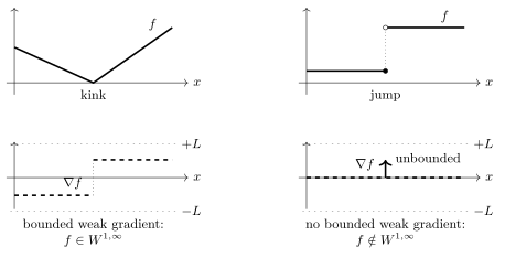
A Sobolev space is a set of functions whose
derivatives, taken in a generalized sense, have bounded
size. Machine learning (ML) methods whose hypothesis space is a ball in a Sobolev
space with a bound on the gradient enforce a well-defined
quantitative notion of robustness: any hypothesis map
in such a ball can be locally approximated by a linear map with
bounded slope, so a small change of the features of a
data point changes the prediction by at most a
proportional amount. The generalized derivative is needed
because hypothesis maps such as those of a deep net with
rectified linear unit (ReLU) activation functions have kinks. A decision tree, whose
hypothesis map jumps, belongs to no Sobolev space and admits
no such guarantee. Linear regression whose hypothesis space is a ball in
a Sobolev space, rather than the linear maps, is
nonparametric regression. Sobolev norms also serve as
regularizers, and they describe the reproducing kernel Hilbert space (RKHS) of a
Matérn kernel.
Definition
B-weakderivA weather service forecasts the
maximum temperature of a day from its minimum temperature.
Fig. 1(a) shows the $366$ days of $2024$ at
the station Krems an der Donau of GeoSphere Austria as the data points of a
scatterplot, with
the minimum temperature of a day as its feature and the
maximum temperature as its label, together with three
hypotheses learned from them: the non-linear map of a
deep net with rectified linear unit (ReLU) activation functions, the step
function of a depth-$2$ decision tree, and the curve of
linear regression with a Sobolev penalty term. A trustworthy
forecaster must not change its prediction, the forecast,
abruptly: a thermometer error of half a degree in
the minimum temperature must not move the forecast by several
degrees. Sobolev spaces make this requirement precise. They
consist of the functions whose derivatives have
bounded size (Evans, 2010, Ch. 5). A bound on the
derivative is a bound on how fast the forecast can change.
Figure 1: Forecasting the maximum temperature of a day at Krems an der Donau
from its minimum temperature. (a) Scatterplot of the
$366$ days of $2024$ (circles) and three hypotheses
learned from them: the non-linear map of a deep net with
ReLU activation functions (solid), the step function of a
depth-$2$ decision tree (dashed), and the curve of
linear regression with a Sobolev penalty term (dotted).
(b) The slope of the deep net hypothesis
$\learnthypothesis$ is a step function, its weak
derivative, and stays below the bound
$\lipschitzconstant = 2.44$ (dotted), so a perturbation $\delta$ of the minimum temperature
moves the forecast by at most $2.44\,|\delta|$. The tree has no
such bound: at each of its thresholds (arrows) the forecast
jumps. Data generated by pythondemos/sobolevspace.py
The derivative is understood in a generalized sense,
since the deep net of Fig. 1(a) has kinks
and no classical derivative exists there. The generalized derivative starts from integration instead
of differentiation. On the real line, a function with
$f(x) = f(a) + \int_{a}^{x} g(t) \, \mathrm{d}t$ is the integral of
its slope $g$, the flow accumulated from $a$ to $x$, and $g$ is
called a weak derivative of $f$. On an open set
$\Omega \subseteq \reals^{\nrfeatures}$, a function
$g_{\featureidx}$ is a weak partial derivative of $f$ if, for
every infinitely differentiable $\varphi$ that vanishes
outside a bounded subset of $\Omega$
(Evans, 2010, Sect. 5.2),
\[
\int_{\Omega} f(\featurevec) \frac{\partial \varphi(\featurevec)}{\partial \feature_{\featureidx}} \, \mathrm{d}\featurevec
= - \int_{\Omega} g_{\featureidx}(\featurevec) \varphi(\featurevec) \, \mathrm{d}\featurevec \text{.}
\]
This is integration by parts with all derivatives moved onto
$\varphi$. It holds when $f$ is the integral of $g_{\featureidx}$
along the $\featureidx$th coordinate, and it never asks for a
derivative of $f$ at a particular point. The slope of the deep net, the step
function of Fig. 1(b), satisfies it for
every test function tried
(pythondemos/sobolevspace.py). For $p \in [1,\infty]$, the
Sobolev space $W^{1,p}(\Omega)$ consists of the functions
whose weak derivatives exist and have finite $L^{p}$
norm $\normgeneric{\cdot}{p}$. The case $p = 2$ gives the
Hilbert space $H^{1}(\Omega)$, and the spaces $W^{k,p}(\Omega)$
require weak derivatives up to order $k$
(Adams and Fournier, 2003, Ch. 3).
B-lipschitzThe case that matters most for machine learning (ML) is $W^{1,\infty}$, the
functions with a bounded weak gradient. A
function $f$ belongs to it with
$\sup_{\featurevec \in \Omega} \normgeneric{\nabla f(\featurevec)}{2} \leq \lipschitzconstant$
precisely when it is Lipschitz continuous with constant
$\lipschitzconstant$ (Evans, 2010, Sect. 5.8). Perturbing a
feature vector by $\boldsymbol{\delta}$ then changes $f$ by at
most $\lipschitzconstant \normgeneric{\boldsymbol{\delta}}{2}$. The
deep net of Fig. 1 has
$\lipschitzconstant = 2.44$, so an error of $0.5\,^{\circ}$C in the
minimum temperature moves its forecast by at most
$1.22\,^{\circ}$C; the largest change among $20000$ random
perturbations of that size was $1.21\,^{\circ}$C.
B-locallinearThe bound also says that near almost every feature vector the hypothesis
agrees with a linear map whose slope is at most
$\lipschitzconstant$ (Rademacher's theorem,
Evans, 2010, Sect. 5.8). This linear map is the
explanation that gradient-based explainable artificial intelligence (XAI) delivers and
that local interpretable model-agnostic explanations (LIME) fits from perturbed data points. For the
forecast, it reads: one additional degree in the minimum adds
$s(x)$ degrees to the forecast, with the slope $s(x)$ of
Fig. 1(b) between $0$ and $2.44$. Since the
deep net is piecewise linear, the approximation is exact
whenever no kink lies between $x$ and $x + \delta$, which was the
case for $98.0\%$ of $20000$ random pairs with
$|\delta| \leq 0.1\,^{\circ}$C. The guarantee comes from the bound,
not from the space: $W^{1,\infty}$ contains functions with
every value of $\lipschitzconstant$. An ML method whose
hypothesis space is the ball of functions with slope at most
$\lipschitzconstant$ learns a robust hypothesis by
construction, whatever the training set. The choice $p = \infty$
is what makes the bound hold at every feature vector; $H^{1}$
bounds the slope only on average.
B-spectralFor the deep net, the weak gradient is bounded by the
product of the spectral norms of its weight matrices, i.e.,
of their largest singular values, here $46.0$ against the true $2.44$: valid but loose.
For a classifier that takes the sign of such an $f$, the
bound certifies that no perturbation of Euclidean norm below
$|f(\featurevec)|/\lipschitzconstant$ changes the prediction
(Tsuzuku et al., 2018). The decision tree of
Fig. 1(a) has no such bound: at its root
threshold of $5.5\,^{\circ}$C, a change of
$2 \cdot 10^{-9}\,^{\circ}$C in the minimum temperature moves the
forecast by $7.81\,^{\circ}$C. A jump has no weak derivative
that is a function, so no Sobolev space contains the tree.
The bound concerns perturbations of the features only;
robustness against perturbations of the training set is a
property of the training map (see stability).
B-nonparamSobolev spaces also serve as hypothesis spaces in their own right.
Plain linear regression minimizes the average squared error loss over the
linear maps. Replacing the linear maps by a ball in $H^{1}$, or
equivalently adding the squared $H^{1}$ seminorm
$\int_{\Omega} \normgeneric{\nabla f(\featurevec)}{2}^{2} \, \mathrm{d}\featurevec$
as a penalty term, a norm that ignores constant shifts of
$f$ (see regularization), gives
nonparametric regression (Wainwright, 2019, Ch. 13). The
dotted curve of Fig. 1(a) minimizes the
training error plus ten times that seminorm; it reaches a
training error of $18.03$, below the $18.66$ of the deep net,
with slope at most $3.05$ (pythondemos/sobolevspace.py).
A computer cannot search all of $H^{1}$, and it need not. A
minimizer of the training error plus the seminorm is piecewise
linear with kinks at the $\samplesize$ data points, since
between two data points the straight line has the smallest
seminorm for given end values (a consequence of the Cauchy–Schwarz
inequality). The search therefore runs over
$\samplesize$ numbers, the values at the kinks; this is
kernel ridge regression with the reproducing kernel Hilbert space (RKHS) of $H^{1}$
(Wainwright, 2019, Ch. 12). For a piecewise linear
function the seminorm is a sum of squared slopes, one per
segment and weighted by its length, so the
normal equations of the penalized problem form one linear
system. The demo places the kinks on $200$ equally spaced points
instead of the data points, which changes nothing in the
arithmetic.
B-graphThe seminorm expresses the smoothness assumption. Its
counterpart for a function on the nodes of a graph
replaces the gradient by differences across edges, the form
used by generalized total variation (GTV) and generalized total variation minimization (GTVMin) (SarcheshmehPour et al., 2023);
penalizing the gradient in $L^{1}$ instead gives total variation
regularization, which allows jumps
(Rudin et al., 1992). The RKHS of a Matérn
kernel is a Sobolev space $W^{s,2}(\Omega)$ whose order $s$
is set by the smoothness parameter of the kernel
(Kanagawa et al., 2018, Example 2.6). A kernel method with
that kernel is therefore again nonparametric
regression over a Sobolev ball, the setting of
(Wainwright, 2019, Ch. 13) above.
Finally, a bound $\lipschitzconstant$ is also of regulatory interest.
Article 15 of the EU AI Act requires a high-risk artificial intelligence system (high-risk AI system)
to be robust and to have its accuracy metrics declared in the
instructions for use (European Parliament and Council of the European Union, 2024). A Lipschitz constant is
such a metric: it states, as a single number, how much a
perturbation of a feature vector can change the prediction.
Evans (2010). Partial Differential Equations. American Mathematical Society.
Adams and Fournier (2003). Sobolev Spaces. Academic Press.
Tsuzuku et al. (2018). Lipschitz-Margin Training: Scalable Certification of Perturbation Invariance for Deep Neural Networks. Adv. Neural Inf. Process. Syst. (NeurIPS).
Wainwright (2019). High-Dimensional Statistics: A Non-Asymptotic Viewpoint. Cambridge University Press.
SarcheshmehPour et al. (2023). Clustered Federated Learning via Generalized Total Variation Minimization. IEEE Trans. Signal Process.. doi.org/10.1109/TSP.2023.3322848
Rudin et al. (1992). Nonlinear total variation based noise removal algorithms. Physica D: Nonlinear Phenomena.
Kanagawa et al. (2018). Gaussian Processes and Kernel Methods: A Review on Connections and Equivalences. arxiv.org/abs/1807.02582
European Parliament and Council of the European Union (2024). Regulation (EU) 2024/1689 of the European Parliament and of the Council of 13 June 2024 laying down harmonised rules on artificial intelligence and amending Regulations (EC) No 300/2008, (EU) No 167/2013, (EU) No 168/2013, (EU) 2018/858, (EU) 2018/1139 and (EU) 2019/2144 and Directives 2014/90/EU, (EU) 2016/797 and (EU) 2020/1828 (Artificial Intelligence Act) (Text with EEA relevance). eur-lex.europa.eu/eli/reg/2024/1689/oj/eng
Cite this entry
@misc{dictml_sobolevspace,
  author = {Jung, Alexander},
  editor = {Olioumtsevits, Konstantina and Schnoor, Ekkehard},
  title = {Sobolev space},
  howpublished = {Dictionary of Applied Machine Learning (course edition)},
  year = {2026},
  doi = {10.5281/zenodo.21569296},
  note = {ISBN 978-952-64-3013-3, CC BY 4.0, retrieved 2026-10-05},
  url = {https://dictionaryofml.org/terms/sobolevspace.html}
}