B-graph writes when the script runsDictionary of Applied Machine Learning · Sobolev space
Numerical companion to the entry Sobolev space: it recomputes what the entry states and prints one line per check
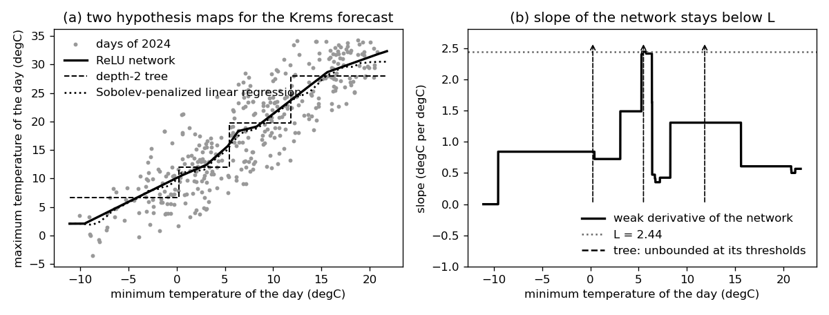
Running example: forecast the maximum temperature of a day at the GeoSphere station Krems (station id 3805) from its minimum temperature. A deep ReLU network learns a non-linear hypothesis map from the 366 days of 2024; a depth-2 decision tree learns a piecewise constant one on the same data. Every claim of the entry is verified on these two maps: the integration-by-parts identity of the weak derivative, the equivalence "bounded weak gradient <=> Lipschitz", the robustness reading of that bound, the spectral-norm bound for the network, the absence of any such bound for the tree, and the two regularizers built from Sobolev seminorms. Self-contained (numpy/matplotlib only), fixed seeds.
Run it without installing anything:uv run https://dictionaryofml.org/terms/sobolevspace.py
uv downloads this script and the pinned NumPy and Matplotlib it needs, then runs it; the script fetches any input file it uses. To keep the output files, download sobolevspace.py into a folder and run uv run sobolevspace.py there. With NumPy and Matplotlib already installed, python3 sobolevspace.py, from any directory — it writes its output files into the current directory. Fixed seeds, so the printed numbers reproduce exactly. Download sobolevspace.py · Notebook · Open in Colab
One cell per block of the script: the code, and what that code printed when it last ran here
"""
sobolevspace.py — numerical companion to the glossary entry 'Sobolev space'.

Running example: forecast the maximum temperature of a day at the
GeoSphere station Krems (station id 3805) from its minimum temperature.
A deep ReLU network learns a non-linear hypothesis map from the 366 days
of 2024; a depth-2 decision tree learns a piecewise constant one on the
same data.  Every claim of the entry is verified on these two maps: the
integration-by-parts identity of the weak derivative, the equivalence
"bounded weak gradient <=> Lipschitz", the robustness reading of that
bound, the spectral-norm bound for the network, the absence of any such
bound for the tree, and the two regularizers built from Sobolev
seminorms.  Self-contained (numpy/matplotlib only), fixed seeds.

Blocks
------
[B-forecast]  Download the 366 days of 2024 at Krems (tlmin, tlmax) and
              train a ReLU network with three hidden layers of width 8
              by gradient descent on the squared error loss.  The learned map is
              non-linear: its slope varies across the feature range.
[B-weakderiv] The network is piecewise linear, so its classical
              derivative is undefined at the kinks.  Its slope g, a
              step function, satisfies the defining identity
              int f(x) phi'(x) dx = - int g(x) phi(x) dx for infinitely
              differentiable test functions phi vanishing at both
              ends: g is the weak
              derivative of f.
[B-lipschitz] The largest value of |g| equals the largest difference
              quotient |f(x) - f(x')| / |x - x'| to three decimals: a
              bounded weak derivative IS a Lipschitz constant L.  Hence
              a perturbation delta of the minimum temperature moves the
              forecast by at most L |delta|; 20000 random perturbations
              of up to 0.5 degC confirm the bound.
[B-locallinear] Near almost every minimum temperature x the forecast
              agrees with the linear map x + delta -> f(x) + g(x) delta:
              for 20000 random pairs with |delta| <= 0.1 degC the
              first-order error is exactly zero whenever no kink lies
              between x and x + delta, and never exceeds 2 L |delta|.
[B-spectral]  The product of the largest singular values of the weight
              matrices bounds L (valid but loose).
[B-jump]      The depth-2 tree is piecewise constant with jumps: a
              perturbation of 2e-9 degC across its root threshold moves
              the forecast by the jump height.  No constant L exists.
[B-nonparam]  Linear regression with a Sobolev penalty (nonparametric
              regression): the squared error loss over piecewise linear maps on
              200 knots with the penalty lambda * int f'^2, solved as one
              linear system.  Raising lambda lowers the H^1 energy of the
              fit and raises its training error; the fit's slope stays
              below a bound L of its own.
[B-tvh1]      Sharpening a transition of width eps: the squared H^1
              seminorm grows like 4 / (3 eps) while the total variation
              stays at the height of the limiting jump — why the L^1
              gradient penalty tolerates jumps and the H^1 penalty does
              not.
[B-graph]     Graph counterpart: for node values sampled from a sine
              the edge-difference energy (the Laplacian
              quadratic form used by GTVMin) is small, while node values
              with one jump make it large.

Outputs
-------
sobolevspace_weather.csv : date, tmin, tmax of the 366 downloaded days
sobolevspace_scatter.csv : tmin, tmax of the 366 days
sobolevspace_net.csv     : tmin, pred, slope at the breakpoints of the network
sobolevspace_tree.csv    : tmin, pred -- the tree's step function
sobolevspace_spline.csv  : tmin, pred -- the Sobolev-penalized linear regression fit
sobolevspace.png         : preview (checking only)
"""

import json
import urllib.request
from pathlib import Path

import numpy as np
import matplotlib

matplotlib.use("Agg")
import matplotlib.pyplot as plt

OUT_DIR = Path(__file__).parent

report = []                         # collects (check name, pass/fail) pairs


def check(name, ok):                # records and prints one verification
    report.append((name, bool(ok)))
    print(f"  [{'ok' if ok else 'FAIL'}] {name}")
Download the 366 days of 2024 at Krems (tlmin, tlmax) and train a ReLU network with three hidden layers of width 8 by gradient descent on the squared error loss. The learned map is non-linear: its slope varies across the feature range.
print("[B-forecast] download the Krems data and train the network")
URL = ("https://dataset.api.hub.geosphere.at/v1/station/historical/"
       "klima-v2-1d?parameters=tlmin,tlmax&station_ids=3805"
       "&start=2024-01-01&end=2024-12-31")
with urllib.request.urlopen(URL, timeout=120) as resp:
    payload = json.load(resp)
params = payload["features"][0]["properties"]["parameters"]
records = [(stamp[:10], lo, hi)
           for stamp, lo, hi in zip(payload["timestamps"],
                                    params["tlmin"]["data"],
                                    params["tlmax"]["data"])
           if lo is not None and hi is not None]
with open(OUT_DIR / "sobolevspace_weather.csv", "w") as f:
    f.write("date,tmin,tmax\n")
    for day, lo, hi in records:
        f.write(f"{day},{lo},{hi}\n")
check(f"[B-forecast] {len(records)} days downloaded for 2024", len(records) == 366)

tmin = np.array([lo for _, lo, _ in records], dtype=float)
tmax = np.array([hi for _, _, hi in records], dtype=float)
np.savetxt(OUT_DIR / "sobolevspace_scatter.csv", np.stack([tmin, tmax], 1),
           delimiter=",", header="tmin,tmax", comments="", fmt="%.1f")

mu_x, sd_x = tmin.mean(), tmin.std()
mu_y, sd_y = tmax.mean(), tmax.std()
Z = ((tmin - mu_x) / sd_x)[:, None]           # standardized feature
Y = ((tmax - mu_y) / sd_y)[:, None]           # standardized label

rng = np.random.default_rng(20260918)
WIDTHS = [1, 8, 8, 8, 1]
Ws = [rng.normal(size=(a, b)) * np.sqrt(2.0 / a)
      for a, b in zip(WIDTHS[:-1], WIDTHS[1:])]
bs = [np.zeros(b) for b in WIDTHS[1:]]


def forward(Zin):
    """Return the output and the ReLU masks of the hidden layers."""
    a, masks = Zin, []
    for W, b in zip(Ws[:-1], bs[:-1]):
        pre = a @ W + b
        masks.append(pre > 0)
        a = np.maximum(pre, 0.0)
    return a @ Ws[-1] + bs[-1], masks


# gradient descent on the average squared error loss over all 366 days
LR = 0.1
for step in range(5000):
    acts, masks = [Z], []
    a = Z
    for W, b in zip(Ws[:-1], bs[:-1]):
        pre = a @ W + b
        masks.append(pre > 0)
        a = np.maximum(pre, 0.0)
        acts.append(a)
    out = a @ Ws[-1] + bs[-1]
    delta = 2.0 * (out - Y) / len(Y)                     # d loss / d out
    grads_w, grads_b = [], []
    for layer in range(len(Ws) - 1, -1, -1):
        grads_w.insert(0, acts[layer].T @ delta)
        grads_b.insert(0, delta.sum(0))
        if layer > 0:
            delta = (delta @ Ws[layer].T) * masks[layer - 1]
    for k in range(len(Ws)):
        Ws[k] -= LR * grads_w[k]
        bs[k] -= LR * grads_b[k]


def f_net(x):
    """Forecast of tmax (degC) for minimum temperatures x (degC)."""
    out, _ = forward(((np.asarray(x, dtype=float) - mu_x) / sd_x)[:, None])
    return out[:, 0] * sd_y + mu_y


def slope_net(x):
    """Weak derivative of f_net at x (degC per degC), read off the masks."""
    _, masks = forward(((np.asarray(x, dtype=float) - mu_x) / sd_x)[:, None])
    J = np.repeat(Ws[0], len(x), axis=0)                 # (n, width)
    for k, mask in enumerate(masks):
        J = (J * mask) @ Ws[k + 1] if k + 1 < len(Ws) - 1 else (J * mask) @ Ws[-1]
    return J[:, 0] * sd_y / sd_x


grid = np.linspace(tmin.min() - 1.0, tmin.max() + 1.0, 40001)
pred, slope = f_net(grid), slope_net(grid)
err_net = float(np.mean((tmax - f_net(tmin)) ** 2))
check(f"[B-forecast] the learned map is non-linear: its slope ranges from "
      f"{slope.min():.2f} to {slope.max():.2f} degC per degC",
      slope.max() - slope.min() > 0.1)
print(f"  average squared error loss of the network on the 366 days: {err_net:.2f}")
# the map is piecewise linear: its breakpoints describe it exactly
kinks = np.flatnonzero(np.diff(slope) != 0.0)
keep = np.unique(np.concatenate([[0], kinks, kinks + 1, [len(grid) - 1]]))
np.savetxt(OUT_DIR / "sobolevspace_net.csv",
           np.stack([grid[keep], pred[keep], slope[keep]], 1),
           delimiter=",", header="tmin,pred,slope", comments="", fmt="%.4f")
[B-forecast] download the Krems data and train the network
  [ok] [B-forecast] 366 days downloaded for 2024
  [ok] [B-forecast] the learned map is non-linear: its slope ranges from 0.00 to 2.44 degC per degC
  average squared error loss of the network on the 366 days: 18.66
The network is piecewise linear, so its classical derivative is undefined at the kinks. Its slope g, a step function, satisfies the defining identity int f(x) phi'(x) dx = - int g(x) phi(x) dx for infinitely differentiable test functions phi vanishing at both ends: g is the weak derivative of f.
print("[B-weakderiv] integration-by-parts identity for the network")
a_, b_ = grid[0], grid[-1]
for p in (1, 2, 3):
    # infinitely differentiable test function vanishing at both ends
    phi = np.sin(p * np.pi * (grid - a_) / (b_ - a_))
    dphi = p * np.pi / (b_ - a_) * np.cos(p * np.pi * (grid - a_) / (b_ - a_))
    lhs = np.trapezoid(pred * dphi, grid)
    rhs = -np.trapezoid(slope * phi, grid)
    check(f"[B-weakderiv] int f phi' = -int g phi for phi_{p} "
          f"({lhs:.4f} vs {rhs:.4f})", abs(lhs - rhs) < 1e-2 * max(1.0, abs(lhs)))
[B-weakderiv] integration-by-parts identity for the network
  [ok] [B-weakderiv] int f phi' = -int g phi for phi_1 (-21.8458 vs -21.8459)
  [ok] [B-weakderiv] int f phi' = -int g phi for phi_2 (2.1526 vs 2.1526)
  [ok] [B-weakderiv] int f phi' = -int g phi for phi_3 (-3.2760 vs -3.2760)
The largest value of |g| equals the largest difference quotient |f(x) - f(x')| / |x - x'| to three decimals: a bounded weak derivative IS a Lipschitz constant L. Hence a perturbation delta of the minimum temperature moves the forecast by at most L |delta|; 20000 random perturbations of up to 0.5 degC confirm the bound.
print("[B-lipschitz] the bound on the weak derivative is a robustness guarantee")
L_emp = float(np.abs(slope).max())
i = rng.integers(0, len(grid), 30000)
j = rng.integers(0, len(grid), 30000)
sep = np.abs(grid[i] - grid[j]); ok = sep > 1e-9
quot = float(np.max(np.abs(pred[i][ok] - pred[j][ok]) / sep[ok]))
check(f"[B-lipschitz] sup |weak derivative| ({L_emp:.3f}) equals the largest "
      f"difference quotient ({quot:.3f})", abs(L_emp - quot) < 2e-3)
x0 = rng.uniform(tmin.min(), tmin.max(), 20000)
dlt = rng.uniform(-0.5, 0.5, 20000)
change = np.abs(f_net(x0 + dlt) - f_net(x0))
check(f"[B-lipschitz] 20000 perturbations of up to 0.5 degC: every forecast "
      f"change <= L |delta| (largest {change.max():.3f} <= {0.5 * L_emp:.3f})",
      np.all(change <= L_emp * np.abs(dlt) + 1e-9))
[B-lipschitz] the bound on the weak derivative is a robustness guarantee
  [ok] [B-lipschitz] sup |weak derivative| (2.441) equals the largest difference quotient (2.441)
  [ok] [B-lipschitz] 20000 perturbations of up to 0.5 degC: every forecast change <= L |delta| (largest 1.213 <= 1.220)
Near almost every minimum temperature x the forecast agrees with the linear map x + delta -> f(x) + g(x) delta: for 20000 random pairs with |delta| <= 0.1 degC the first-order error is exactly zero whenever no kink lies between x and x + delta, and never exceeds 2 L |delta|.
print("[B-locallinear] first-order approximation of the forecast")
x1 = rng.uniform(tmin.min(), tmin.max(), 20000)
d1 = rng.uniform(-0.1, 0.1, 20000)
err1 = np.abs(f_net(x1 + d1) - f_net(x1) - slope_net(x1) * d1)
k_lo, k_hi = grid[kinks], grid[kinks + 1]             # grid cells holding a kink
lo_, hi_ = np.minimum(x1, x1 + d1), np.maximum(x1, x1 + d1)
crossed = np.array([np.any((k_hi > lo) & (k_lo < hi)) for lo, hi in zip(lo_, hi_)])
check(f"[B-locallinear] the approximation is exact when no kink lies between x "
      f"and x + delta ({100 * (1 - crossed.mean()):.1f}% of the pairs)",
      np.all(err1[~crossed] < 1e-9))
check(f"[B-locallinear] across a kink the error stays below 2 L |delta| "
      f"(largest ratio {np.max(err1 / (2 * L_emp * np.abs(d1))):.3f})",
      np.all(err1 <= 2 * L_emp * np.abs(d1) + 1e-9))
[B-locallinear] first-order approximation of the forecast
  [ok] [B-locallinear] the approximation is exact when no kink lies between x and x + delta (98.0% of the pairs)
  [ok] [B-locallinear] across a kink the error stays below 2 L |delta| (largest ratio 0.323)
The product of the largest singular values of the weight matrices bounds L (valid but loose).
print("[B-spectral] spectral-norm bound on the weak derivative")
L_spec = float(np.prod([np.linalg.norm(W, 2) for W in Ws]) * sd_y / sd_x)
check(f"[B-spectral] product of largest singular values bounds L: "
      f"{L_emp:.3f} <= {L_spec:.3f}", L_emp <= L_spec + 1e-9)
[B-spectral] spectral-norm bound on the weak derivative
  [ok] [B-spectral] product of largest singular values bounds L: 2.441 <= 46.019
The depth-2 tree is piecewise constant with jumps: a perturbation of 2e-9 degC across its root threshold moves the forecast by the jump height. No constant L exists.
print("[B-jump] the tree's forecast jumps")
MINLEAF = 5


def best_split(x, y):
    order = np.argsort(x)
    xs, ys = x[order], y[order]
    best, best_sse = None, np.inf
    for k in range(MINLEAF, len(xs) - MINLEAF + 1):
        if xs[k - 1] == xs[k]:
            continue
        left, right = ys[:k], ys[k:]
        sse = ((left - left.mean()) ** 2).sum() + ((right - right.mean()) ** 2).sum()
        if sse < best_sse:
            best_sse, best = sse, (xs[k - 1] + xs[k]) / 2
    return best


root_t = best_split(tmin, tmax)
cuts = [root_t]
for side in (tmin <= root_t, tmin > root_t):
    t = best_split(tmin[side], tmax[side])
    if t is not None:
        cuts.append(t)
cuts = sorted(cuts)
edges = [-np.inf] + cuts + [np.inf]
means = np.array([tmax[(tmin > lo) & (tmin <= hi)].mean()
                  for lo, hi in zip(edges[:-1], edges[1:])])
f_tree = lambda xq: means[np.searchsorted(np.array(cuts), np.asarray(xq, dtype=float))]
eps = 1e-9
jump = float(abs(f_tree([root_t + eps]) - f_tree([root_t - eps]))[0])
check(f"[B-jump] across the root threshold {root_t:.2f} degC a perturbation of "
      f"{2 * eps:.0e} degC moves the forecast by {jump:.2f} degC — no constant L",
      jump > 1.0)
bounds = [tmin.min() - 1.0] + cuts + [tmin.max() + 1.0]
rows = []
for lo, hi, mv in zip(bounds[:-1], bounds[1:], means):
    rows += [(lo, mv), (hi, mv)]
np.savetxt(OUT_DIR / "sobolevspace_tree.csv", np.array(rows),
           delimiter=",", header="tmin,pred", comments="", fmt="%.4f")
[B-jump] the tree's forecast jumps
  [ok] [B-jump] across the root threshold 5.50 degC a perturbation of 2e-09 degC moves the forecast by 7.81 degC — no constant L
Linear regression with a Sobolev penalty (nonparametric regression): the squared error loss over piecewise linear maps on 200 knots with the penalty lambda * int f'^2, solved as one linear system. Raising lambda lowers the H^1 energy of the fit and raises its training error; the fit's slope stays below a bound L of its own.
print("[B-nonparam] squared error loss over piecewise linear maps with the H^1 penalty")
knots = np.linspace(tmin.min() - 1.0, tmin.max() + 1.0, 200)
h_k = knots[1] - knots[0]
idx = np.clip(np.searchsorted(knots, tmin) - 1, 0, len(knots) - 2)
wgt = (tmin - knots[idx]) / h_k
S_mat = np.zeros((len(tmin), len(knots)))          # piecewise linear map at the days
S_mat[np.arange(len(tmin)), idx] = 1.0 - wgt
S_mat[np.arange(len(tmin)), idx + 1] = wgt
D_mat = (np.eye(len(knots))[1:] - np.eye(len(knots))[:-1]) / h_k   # slopes between knots


def spline_fit(lam):
    """Knot values minimizing sum (y - f(x))^2 + lam * int f'(x)^2 dx."""
    A = S_mat.T @ S_mat + lam * h_k * D_mat.T @ D_mat
    return np.linalg.solve(A, S_mat.T @ tmax)


h1_energy = lambda v: float(h_k * np.sum((D_mat @ v) ** 2))
fits = {lam: spline_fit(lam) for lam in (1.0, 10.0, 100.0)}
energies = [h1_energy(v) for v in fits.values()]
errors = [float(np.mean((tmax - S_mat @ v) ** 2)) for v in fits.values()]
check("[B-nonparam] a larger penalty weight lowers the H^1 energy of the fit "
      f"({', '.join(f'{e:.1f}' for e in energies)})",
      all(b < a for a, b in zip(energies, energies[1:])))
check("[B-nonparam] and raises its training error "
      f"({', '.join(f'{e:.2f}' for e in errors)})",
      all(b > a for a, b in zip(errors, errors[1:])))
v_sp = fits[10.0]
L_sp = float(np.abs(D_mat @ v_sp).max())
print(f"  penalty weight 10: training error {errors[1]:.2f}, largest slope {L_sp:.2f} degC per degC")
np.savetxt(OUT_DIR / "sobolevspace_spline.csv", np.stack([knots, v_sp], 1),
           delimiter=",", header="tmin,pred", comments="", fmt="%.4f")
[B-nonparam] squared error loss over piecewise linear maps with the H^1 penalty
  [ok] [B-nonparam] a larger penalty weight lowers the H^1 energy of the fit (300.8, 40.1, 22.5)
  [ok] [B-nonparam] and raises its training error (16.43, 18.03, 19.55)
  penalty weight 10: training error 18.03, largest slope 3.05 degC per degC
Sharpening a transition of width eps: the squared H^1 seminorm grows like 4 / (3 eps) while the total variation stays at the height of the limiting jump — why the L^1 gradient penalty tolerates jumps and the H^1 penalty does not.
print("[B-tvh1] squared H^1 seminorm vs total variation of a sharpening transition")
xs = np.linspace(-3.0, 3.0, 600001)
h1, tv = [], []
for width in (0.2, 0.05, 0.0125):
    df = (1.0 / width) / np.cosh(xs / width) ** 2     # derivative of tanh(x/width)
    h1.append(np.trapezoid(df ** 2, xs))              # squared H^1 seminorm
    tv.append(np.trapezoid(np.abs(df), xs))           # total variation
check("[B-tvh1] H^1 energy grows without bound as the transition sharpens "
      f"({', '.join(f'{v:.1f}' for v in h1)})",
      all(b > 3.5 * a for a, b in zip(h1, h1[1:])))
check("[B-tvh1] total variation stays at the height of the jump "
      f"({', '.join(f'{v:.4f}' for v in tv)})",
      all(abs(v - 2.0) < 1e-3 for v in tv))
[B-tvh1] squared H^1 seminorm vs total variation of a sharpening transition
  [ok] [B-tvh1] H^1 energy grows without bound as the transition sharpens (6.7, 26.7, 106.7)
  [ok] [B-tvh1] total variation stays at the height of the jump (2.0000, 2.0000, 2.0000)
Graph counterpart: for node values sampled from a sine the edge-difference energy (the Laplacian quadratic form used by GTVMin) is small, while node values with one jump make it large.
print("[B-graph] edge-difference energy on a chain graph")
n = 60
nodes = np.linspace(0.0, 1.0, n)
chain = [(k, k + 1) for k in range(n - 1)]          # chain of nodes, unit weights
smooth = np.sin(2 * np.pi * nodes)                  # samples of a sine
jumpy = np.where(nodes < 0.5, -1.0, 1.0)            # one jump of height 2
energy = lambda s: sum((s[a] - s[b]) ** 2 for a, b in chain)
check(f"[B-graph] edge-difference energy: sine node values {energy(smooth):.4f} "
      f"<< node values with one jump {energy(jumpy):.4f}",
      energy(smooth) < 0.1 * energy(jumpy))

# ---- preview figure (checking only)
fig, (ax1, ax2) = plt.subplots(1, 2, figsize=(10, 3.8))
ax1.plot(tmin, tmax, "o", ms=2.5, color="0.6", label="days of 2024")
ax1.plot(grid, pred, "-", color="black", lw=2, label="ReLU network")
tr = np.array(rows)
ax1.plot(tr[:, 0], tr[:, 1], "--", color="black", lw=1.2, label="depth-2 tree")
ax1.plot(knots, v_sp, ":", color="black", lw=1.6, label="Sobolev-penalized linear regression")
ax1.set_xlabel("minimum temperature of the day (degC)")
ax1.set_ylabel("maximum temperature of the day (degC)")
ax1.set_title("(a) two hypothesis maps for the Krems forecast")
ax1.legend(frameon=False, loc="upper left")
ax2.plot(grid, slope, "-", color="black", lw=2, label="weak derivative of the network")
ax2.axhline(L_emp, ls=":", color="0.4", label=f"L = {L_emp:.2f}")
for c in cuts:
    ax2.annotate("", xy=(c, 2.6), xytext=(c, 0.0),
                 arrowprops=dict(arrowstyle="->", color="black", ls="--"))
ax2.plot([], [], "--", color="black", label="tree: unbounded at its thresholds")
ax2.set_xlabel("minimum temperature of the day (degC)")
ax2.set_ylabel("slope (degC per degC)")
ax2.set_ylim(-1.0, 2.8)
ax2.set_title("(b) slope of the network stays below L")
ax2.legend(frameon=False, loc="lower right")
fig.tight_layout()
fig.savefig(OUT_DIR / "sobolevspace.png", dpi=120)

n_ok = sum(ok for _, ok in report)
print(f"\n{n_ok}/{len(report)} checks pass")
if n_ok != len(report):
    raise SystemExit(1)
[B-graph] edge-difference energy on a chain graph
  [ok] [B-graph] edge-difference energy: sine node values 0.3342 << node values with one jump 4.0000

16/16 checks pass
B-graph writes when the script runs