Dictionary of Applied Machine Learning
Updated on 2026-10-02
Typeset PDF version — the authoritative form of this entry
Python demo — a script that recomputes what this entry states and prints one line per check
The bootstrap estimates how much the output of a machine learning (ML) method moves when its dataset is drawn again, using only the one dataset at hand. It reads the data points as realizations of independent and identically distributed (i.i.d.) random variables (RVs) and replaces their unknown probability distribution by the empirical distribution of the dataset, so that drawing a new dataset becomes drawing with replacement from the old one. Each of the $\nrbootstraps$ datasets so drawn has the same size as the original, repeats some data points and omits others, and holds about $0.63\,\samplesize$ distinct ones. Model training on each gives $\nrbootstraps$ learned hypotheses whose spread estimates the variance of the method. Resampling a test set with replacement, with the learned hypothesis held fixed, gives a confidence interval for a reported accuracy. The overlap with the original dataset is what distinguishes the bootstrap from $k$-fold cross-validation ($k$-fold CV), whose blocks do not overlap, and it makes a naive bootstrap estimate of prediction error optimistic. Bootstrap aggregating (bagging) puts the same resampling to a different use, averaging the hypotheses instead of measuring their spread.
Forty days of weather recordings fix one straight line through them. Had forty other days been recorded, the line would have come out slightly different, and how much it would move is what decides whether its slope means anything. Only one set of forty days was ever recorded, so the repetitions that would answer the question do not exist. The bootstrap manufactures them from the forty days in hand.
B-empdistTo manufacture them, the forty days are read as realizations of independent and identically distributed (i.i.d.) random variables (RVs). A dataset $\dataset = \big\{ \datapoint^{(1)}, \,\ldots, \,\datapoint^{(\samplesize)}\big\}$ is then a draw of $\samplesize$ such RVs with a common probability distribution $\probdist$. That $\probdist$ is unknown and must be estimated from $\dataset$ itself. The bootstrap estimates it by the empirical distribution $\probdist^{(\dataset)}$ of $\dataset$ (Efron, 1979; Efron and Tibshirani, 1993; Hastie et al., 2009, Sect. 7.11), \[ \frac{1}{\samplesize} \big| \sampleidx: \datapoint^{(\sampleidx)} \in \mathcal{A} \big| \approx \prob{\mathcal{A}} \text{.} \] Once $\probdist$ has been replaced by $\probdist^{(\dataset)}$, the shortage of data is gone: $\probdist^{(\dataset)}$ is a fully specified probability distribution and can be sampled as often as wanted, so as many data points and as many datasets as needed can be generated from the one dataset that was collected. The gain is replicates, not information. Each replicate keeps the size $\samplesize$ of $\dataset$, because the quantity being imitated is the spread of a dataset of that size drawn from $\probdist$. Nor does a replicate reach new data points: $\probdist^{(\dataset)}$ places all its mass on the $\samplesize$ data points observed, so no draw can produce one that $\dataset$ does not already contain.
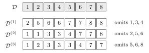
B-fitSampling $\samplesize$ data points from
$\probdist^{(\dataset)}$ is the same as drawing $\samplesize$ times
from $\dataset$ with replacement: every draw is made from the whole
of $\dataset$, so a data point can be drawn twice and another
not at all (Fig. 1). Let
$\nrbootstraps$ be the number of such draws, a number limited only
by the computation they cost. Repeating the draw $\nrbootstraps$
times yields datasets $\dataset^{(1)}, \,\ldots,
\,\dataset^{(\nrbootstraps)}$, each of $\samplesize$
data points.
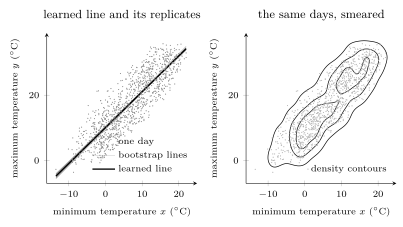
B-testciFig. 2 draws that picture with measured
data: not forty days but $\samplesize = 1096$, the daily minimum
and maximum temperature at Krems an der Donau from $2022$ to
$2024$. In the left panel each dot is one data point, its
feature the minimum temperature and its label the
maximum temperature, and the thick line is the hypothesis
learned from all of them by ERM with the squared error loss.
The thin lines are learned by the same ERM problem from
bootstrap datasets. Their spread is narrow here, and the $95\%$
confidence interval for the slope runs from $1.07$ to $1.13$.
The dots are also all the mass that $\probdist^{(\dataset)}$ has,
which is what the right panel makes visible: smearing each dot into
a small bump and adding the bumps gives a density, and its contours
show two crowded regions, the winter days and the summer days.
Drawing from that smoothed density rather than from the dots is a
variant called the smoothed bootstrap; it produces temperatures
that no day of $\dataset$ recorded, which the bootstrap itself
never does.
pythondemos/bootstrap.py
A data point is left out of a bootstrap dataset with probability $(1 - 1/\samplesize)^{\samplesize}$, so it appears in one with probability $1 - (1 - 1/\samplesize)^{\samplesize}$, which approaches $1 - 1/e \approx 0.63$ as $\samplesize$ grows. A bootstrap dataset therefore holds about $0.63\,\samplesize$ distinct data points and overlaps $\dataset$ heavily. That overlap is what separates the bootstrap from $k$-fold cross-validation ($k$-fold CV), which partitions $\dataset$ into blocks that do not overlap at all. Used naively to estimate prediction error, the bootstrap therefore evaluates the learned hypotheses on data points that entered their own training, and the estimate comes out optimistic (Hastie et al., 2009, Sect. 7.11). The repair is to imitate $k$-fold CV: keep, for each data point, only the predictions of those bootstrap datasets that do not contain it. That leave-one-out bootstrap then trains on about $0.63\,\samplesize$ distinct data points, so its bias behaves like that of $k$-fold CV with $k = 2$, which the $0.632$ estimator corrects (Hastie et al., 2009, Sect. 7.11).
Bootstrap aggregating (bagging) is the bootstrap put to a different use: instead of measuring the spread of $\learnthypothesis^{(1)}, \,\ldots, \,\learnthypothesis^{(\nrbootstraps)}$, it averages them into one hypothesis, which is how a random forest is built from decision trees.
See also: empirical distribution, independent and identically distributed, random variable, probability distribution, variance, $k$-fold cross-validation, bootstrap aggregating, confidence interval, test set, accuracy.
@misc{dictml_bootstrap,
  author = {Jung, Alexander},
  editor = {Olioumtsevits, Konstantina and Schnoor, Ekkehard},
  title = {bootstrap},
  howpublished = {Dictionary of Applied Machine Learning (course edition)},
  year = {2026},
  doi = {10.5281/zenodo.21569296},
  note = {ISBN 978-952-64-3013-3, CC BY 4.0, retrieved 2026-10-02},
  url = {https://dictionaryofml.org/terms/bootstrap.html}
}