B-smooth writes when the script runsDictionary of Applied Machine Learning · bootstrap
Numerical companion to the entry bootstrap: it recomputes what the entry states and prints one line per check
Three years of daily minimum and maximum temperature at Krems an der Donau stand in for the dataset D. The blocks below read those days as realizations of i.i.d. RVs, replace their unknown probability distribution by the empirical distribution of D, and draw from it. Self-contained (numpy/matplotlib only, data fetched from the GeoSphere Austria archive), fixed seed.
Run it without installing anything:uv run https://dictionaryofml.org/terms/bootstrap.py
uv downloads this script and the pinned NumPy and Matplotlib it needs, then runs it; the script fetches any input file it uses. To keep the output files, download bootstrap.py into a folder and run uv run bootstrap.py there. With NumPy and Matplotlib already installed, python3 bootstrap.py, from any directory — it writes its output files into the current directory. Fixed seeds, so the printed numbers reproduce exactly. Download bootstrap.py · Notebook · Open in Colab
One cell per block of the script: the code, and what that code printed when it last ran here
"""
bootstrap.py — numerical companion to the glossary entry 'bootstrap'.

Three years of daily minimum and maximum temperature at Krems an der
Donau stand in for the dataset D. The blocks below read those days as
realizations of i.i.d. RVs, replace their unknown probability
distribution by the empirical distribution of D, and draw from it.
Self-contained (numpy/matplotlib only, data fetched from the GeoSphere
Austria archive), fixed seed.

Blocks
------
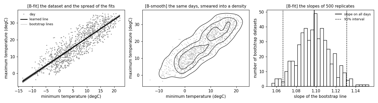
[B-data]    1096 days of (tmin, tmax) at Krems, 2022-2024. This cloud of
            points is the dataset D; the entry's picture of it is the
            scatterplot of the left panel.
[B-empdist] The empirical distribution P^(D) puts mass 1/m on each of
            the m days. Drawing m days from it is drawing from D with
            replacement, and a draw holds about 0.63 m distinct days.
            P^(D) is a complete distribution, so it can be sampled as
            often as wanted: drawing 100 m days from it is no problem,
            and the mean of such a draw converges to the mean of D, not
            to the mean of the unknown P. The gain is replicates, not
            information.
[B-fit]     ERM with the squared error loss fits tmax = w0 + w1 tmin
            on D, which is least squares. Refitting on
            B = 500 bootstrap datasets gives B slopes whose 2.5th to
            97.5th percentile range is a confidence interval for the
            slope; it shrinks like 1/sqrt(m) when m is cut to a quarter.
[B-testci]  A threshold rule predicts a frost night (tmin < 0) from the
            day's tmax. The rule is learned once on a training set and
            its accuracy measured on a held-out test set; resampling
            that test set B times, with the rule held fixed, turns the
            single accuracy into a confidence interval.
[B-smooth]  Smearing each day with a Gaussian kernel turns the m spikes
            of P^(D) into a density estimate, drawn as the contours of
            the right panel. Sampling that density instead of the spikes
            is the smoothed bootstrap: it produces days that D does not
            contain, which the plain bootstrap never does.

Outputs
-------
bootstrap_krems.csv    : tmin, tmax of the 1096 days (figure data).
bootstrap_fit.csv      : the learned line as one two-point segment.
bootstrap_lines.csv    : 25 bootstrap lines, two-point segments separated
                         by empty lines.
bootstrap_density.csv  : contour polylines of the smeared distribution,
                         same separation.
bootstrap.png          : preview figure (checking only).

Data generated by pythondemos/bootstrap.py.
"""

import json
import urllib.request
import numpy as np
import matplotlib

matplotlib.use("Agg")
import matplotlib.pyplot as plt
from pathlib import Path

OUT_DIR = Path(__file__).parent
ARCHIVE = "https://dataset.api.hub.geosphere.at/v1/station/historical/"
STATION = 3805                      # Krems an der Donau
NR_BOOTSTRAP = 500
SEED = 20220101

rng = np.random.default_rng(SEED)
report = []


def check(name, ok):
    report.append((name, bool(ok)))
    print(f"  [{'ok' if ok else 'FAIL'}] {name}")


def fetch(parameters, start, end):
    """Daily parameters of one station from the GeoSphere Austria archive."""
    url = (f"{ARCHIVE}klima-v2-1d?parameters={','.join(parameters)}"
           f"&station_ids={STATION}&start={start}&end={end}")
    with urllib.request.urlopen(url, timeout=180) as resp:
        payload = json.load(resp)
    values = payload["features"][0]["properties"]["parameters"]
    return np.stack([np.array(values[p]["data"], dtype=float)
                     for p in parameters], axis=1)


def least_squares_line(x, y):
    """Slope and intercept of the least-squares fit of y on x."""
    design = np.stack([np.ones_like(x), x], axis=1)
    weights = np.linalg.lstsq(design, y, rcond=None)[0]
    return weights[1], weights[0]


def write_segments(name, header, segments):
    """Polylines, one blank line between them (pgfplots 'empty line=jump')."""
    with open(OUT_DIR / name, "w") as f:
        f.write(header + "\n")
        for k, seg in enumerate(segments):
            if k:
                f.write("\n")
            for px, py in seg:
                f.write(f"{px:.4f},{py:.4f}\n")
1096 days of (tmin, tmax) at Krems, 2022-2024. This cloud of points is the dataset D; the entry's picture of it is the scatterplot of the left panel.
days = fetch(["tlmin", "tlmax"], "2022-01-01", "2024-12-31")
tmin, tmax = days[:, 0], days[:, 1]
m = tmin.size
print(f"[B-data] {m} days at Krems an der Donau, 2022-2024; "
      f"tmin {tmin.min():.1f} to {tmin.max():.1f}, "
      f"tmax {tmax.min():.1f} to {tmax.max():.1f} degrees")
check("[B-data] three full years, no gaps", m == 1096 and not np.isnan(days).any())
with open(OUT_DIR / "bootstrap_krems.csv", "w") as f:
    f.write("tmin,tmax\n")
    for a, b in zip(tmin, tmax):
        f.write(f"{a:.1f},{b:.1f}\n")
[B-data] 1096 days at Krems an der Donau, 2022-2024; tmin -13.5 to 22.0, tmax -3.6 to 35.7 degrees
  [ok] [B-data] three full years, no gaps
The empirical distribution P^(D) puts mass 1/m on each of the m days. Drawing m days from it is drawing from D with replacement, and a draw holds about 0.63 m distinct days. P^(D) is a complete distribution, so it can be sampled as often as wanted: drawing 100 m days from it is no problem, and the mean of such a draw converges to the mean of D, not to the mean of the unknown P. The gain is replicates, not information.
print("[B-empdist] P^(D) puts mass 1/m on each day; drawing from it is "
      "drawing from D with replacement")
idx = rng.integers(0, m, size=m)
check("[B-empdist] a draw of m days holds about 0.63 m distinct days",
      abs(np.unique(idx).size / m - (1 - np.exp(-1.0))) < 0.02)
check("[B-empdist] every drawn day is a day of D",
      np.all(np.isin(tmin[idx], tmin)))
huge = rng.integers(0, m, size=100 * m)
check("[B-empdist] a draw of 100 m days is no problem, and its mean "
      "converges to the mean of D, not to anything new",
      abs(tmax[huge].mean() - tmax.mean()) < 0.1)
check("[B-empdist] such a draw still contains no day outside D",
      np.unique(tmax[huge]).size <= np.unique(tmax).size)
[B-empdist] P^(D) puts mass 1/m on each day; drawing from it is drawing from D with replacement
  [ok] [B-empdist] a draw of m days holds about 0.63 m distinct days
  [ok] [B-empdist] every drawn day is a day of D
  [ok] [B-empdist] a draw of 100 m days is no problem, and its mean converges to the mean of D, not to anything new
  [ok] [B-empdist] such a draw still contains no day outside D
ERM with the squared error loss fits tmax = w0 + w1 tmin on D, which is least squares. Refitting on B = 500 bootstrap datasets gives B slopes whose 2.5th to 97.5th percentile range is a confidence interval for the slope; it shrinks like 1/sqrt(m) when m is cut to a quarter.
slope, intercept = least_squares_line(tmin, tmax)
print(f"[B-fit] tmax = {intercept:.2f} + {slope:.2f} tmin on all {m} days")
slopes = np.empty(NR_BOOTSTRAP)
lines = []
for b in range(NR_BOOTSTRAP):
    draw = rng.integers(0, m, size=m)
    slopes[b], icept = least_squares_line(tmin[draw], tmax[draw])
    if b < 25:
        lines.append([(tmin.min(), icept + slopes[b] * tmin.min()),
                      (tmin.max(), icept + slopes[b] * tmin.max())])
lo, hi = np.percentile(slopes, [2.5, 97.5])
print(f"[B-fit] 95% confidence interval for the slope: [{lo:.3f}, {hi:.3f}]")
check("[B-fit] the interval covers the slope learned from all of D",
      lo <= slope <= hi)
check("[B-fit] the interval is narrow, a few percent of the slope",
      (hi - lo) / slope < 0.12)
quarter = rng.choice(m, size=m // 4, replace=False)
narrow = np.array([least_squares_line(*(lambda d: (tmin[quarter][d],
                                                   tmax[quarter][d]))(
    rng.integers(0, m // 4, size=m // 4)))[0] for _ in range(NR_BOOTSTRAP)])
wide = np.percentile(narrow, 97.5) - np.percentile(narrow, 2.5)
print(f"[B-fit] on a quarter of the days the interval is {wide / (hi - lo):.1f} "
      "times as wide")
check("[B-fit] cutting m to a quarter roughly doubles the interval",
      1.6 < wide / (hi - lo) < 2.6)
# the learned line goes in its own file: the book figure draws it thick and
# the replicates thin, so one file with one style would hide the difference
write_segments("bootstrap_fit.csv", "tmin,tmax",
               [[(tmin.min(), intercept + slope * tmin.min()),
                 (tmin.max(), intercept + slope * tmin.max())]])
write_segments("bootstrap_lines.csv", "tmin,tmax", lines)
[B-fit] tmax = 10.04 + 1.10 tmin on all 1096 days
[B-fit] 95% confidence interval for the slope: [1.067, 1.131]
  [ok] [B-fit] the interval covers the slope learned from all of D
  [ok] [B-fit] the interval is narrow, a few percent of the slope
[B-fit] on a quarter of the days the interval is 2.1 times as wide
  [ok] [B-fit] cutting m to a quarter roughly doubles the interval
A threshold rule predicts a frost night (tmin < 0) from the day's tmax. The rule is learned once on a training set and its accuracy measured on a held-out test set; resampling that test set B times, with the rule held fixed, turns the single accuracy into a confidence interval.
frost = (tmin < 0.0).astype(int)
order = rng.permutation(m)
train, test = order[:800], order[800:]
grid = np.linspace(tmax.min(), tmax.max(), 400)
errors = [(np.mean((tmax[train] <= t).astype(int) != frost[train]), t)
          for t in grid]
threshold = min(errors)[1]
predict = lambda x: (x <= threshold).astype(int)
acc_test = float(np.mean(predict(tmax[test]) == frost[test]))
print(f"[B-testci] threshold {threshold:.1f} degrees learned on "
      f"{train.size} days; accuracy on the {test.size} test days "
      f"{acc_test:.3f}")
check("[B-testci] the learned rule is better than always predicting "
      "no frost", acc_test > 1 - frost[test].mean())
accs = np.array([float(np.mean(predict(tmax[test][d]) == frost[test][d]))
                 for d in rng.integers(0, test.size,
                                       size=(NR_BOOTSTRAP, test.size))])
acc_lo, acc_hi = np.percentile(accs, [2.5, 97.5])
print(f"[B-testci] 95% confidence interval for that accuracy: "
      f"[{acc_lo:.3f}, {acc_hi:.3f}]")
check("[B-testci] the interval covers the measured accuracy",
      acc_lo <= acc_test <= acc_hi)
check("[B-testci] it is several points wide, which the single number "
      "does not show", 0.02 < acc_hi - acc_lo < 0.12)
check("[B-testci] the hypothesis never changes: only the test set is "
      "redrawn", predict(np.array([threshold])).item() == 1)
[B-testci] threshold 7.2 degrees learned on 800 days; accuracy on the 296 test days 0.858
  [ok] [B-testci] the learned rule is better than always predicting no frost
[B-testci] 95% confidence interval for that accuracy: [0.821, 0.897]
  [ok] [B-testci] the interval covers the measured accuracy
  [ok] [B-testci] it is several points wide, which the single number does not show
  [ok] [B-testci] the hypothesis never changes: only the test set is redrawn
Smearing each day with a Gaussian kernel turns the m spikes of P^(D) into a density estimate, drawn as the contours of the right panel. Sampling that density instead of the spikes is the smoothed bootstrap: it produces days that D does not contain, which the plain bootstrap never does.
h_min, h_max = 1.4, 1.8                       # kernel widths, degrees
gx = np.linspace(tmin.min() - 3, tmin.max() + 3, 160)
gy = np.linspace(tmax.min() - 3, tmax.max() + 3, 160)
GX, GY = np.meshgrid(gx, gy)
dens = np.zeros_like(GX)
for a, b in zip(tmin, tmax):
    dens += np.exp(-0.5 * (((GX - a) / h_min) ** 2 + ((GY - b) / h_max) ** 2))
dens /= m * 2 * np.pi * h_min * h_max
cell = (gx[1] - gx[0]) * (gy[1] - gy[0])
print(f"[B-smooth] kernel widths {h_min} and {h_max} degrees; the smeared "
      f"density integrates to {dens.sum() * cell:.3f}")
check("[B-smooth] the density integrates to one", abs(dens.sum() * cell - 1) < 0.02)
counts, edges = np.histogram(tmin, bins=20)
mode_tmin = 0.5 * (edges[counts.argmax()] + edges[counts.argmax() + 1])
peak_tmin = gx[np.unravel_index(dens.argmax(), dens.shape)[1]]
check(f"[B-smooth] its peak ({peak_tmin:.1f} degrees) sits where the days "
      f"pile up ({mode_tmin:.1f}), not at the median ({np.median(tmin):.1f})",
      abs(peak_tmin - mode_tmin) < 1.5)
smoothed = (tmin[rng.integers(0, m, size=20000)]
            + h_min * rng.standard_normal(20000))
check("[B-smooth] the smoothed bootstrap produces days outside D, which "
      "the plain bootstrap never does",
      not np.any(np.isin(smoothed, tmin)))
levels = np.array([0.1, 0.4, 0.7]) * dens.max()

# ------------------------------------------------------------- preview
fig, ax = plt.subplots(1, 3, figsize=(13.2, 3.6))
ax[0].plot(tmin, tmax, ".", color="0.55", markersize=2.5, label="day")
for seg in lines[:25]:
    ax[0].plot([seg[0][0], seg[1][0]], [seg[0][1], seg[1][1]],
               "-", color="0.3", linewidth=0.4)
ax[0].plot([tmin.min(), tmin.max()],
           [intercept + slope * tmin.min(), intercept + slope * tmin.max()],
           "k-", linewidth=1.8, label="learned line")
ax[0].plot([], [], "-", color="0.3", linewidth=0.4, label="bootstrap lines")
ax[0].set_xlabel("minimum temperature (degC)")
ax[0].set_ylabel("maximum temperature (degC)")
ax[0].set_title("[B-fit] the dataset and the spread of the fits", fontsize=10)
ax[0].legend(frameon=False, fontsize=8, loc="upper left")
ax[1].plot(tmin, tmax, ".", color="0.75", markersize=2)
contours = ax[1].contour(GX, GY, dens, levels=levels, colors="black",
                         linewidths=0.9)
# the book figure draws the same contours, so its polylines are taken from
# this panel rather than from a second, throwaway axes
segments = [seg for level in contours.allsegs for seg in level if len(seg) > 8]
write_segments("bootstrap_density.csv", "tmin,tmax", segments)
print(f"[B-smooth] {len(segments)} contour polylines written")
ax[1].set_xlabel("minimum temperature (degC)")
ax[1].set_ylabel("maximum temperature (degC)")
ax[1].set_title("[B-smooth] the same days, smeared into a density",
                fontsize=10)
ax[2].hist(slopes, bins=30, color="white", edgecolor="black")
ax[2].axvline(slope, color="black", linestyle="-", linewidth=1.5,
              label="slope on all days")
ax[2].axvline(lo, color="black", linestyle="--", linewidth=1.0,
              label="95% interval")
ax[2].axvline(hi, color="black", linestyle="--", linewidth=1.0)
ax[2].set_xlabel("slope of the bootstrap line")
ax[2].set_ylabel("number of bootstrap datasets")
ax[2].set_title("[B-fit] the slopes of 500 replicates", fontsize=10)
ax[2].legend(frameon=False, fontsize=8)
fig.tight_layout()
fig.savefig(OUT_DIR / "bootstrap.png", dpi=110)
print(f"\n{sum(ok for _, ok in report)}/{len(report)} checks passed")
assert all(ok for _, ok in report)
[B-smooth] kernel widths 1.4 and 1.8 degrees; the smeared density integrates to 1.000
  [ok] [B-smooth] the density integrates to one
  [ok] [B-smooth] its peak (2.6 degrees) sits where the days pile up (3.4), not at the median (6.8)
  [ok] [B-smooth] the smoothed bootstrap produces days outside D, which the plain bootstrap never does
[B-smooth] 4 contour polylines written

15/15 checks passed
B-smooth writes when the script runs