pythondemos/cav.pyDictionary of Applied Machine Learning
Updated on 2026-10-04
See also feature interpretability transparency explanation explainability
A concept activation vector (CAV) is a direction in the activations of one hidden layer of a deep net that stands for a concept named by a user. The user supplies data points that carry the concept and data points that do not, and a linear classifier is trained to tell the two apart from their activations. The CAV is the direction perpendicular to the hyperplane that separates them, pointing to the concept side. Moving the activations of a data point a little along the CAV changes the score the deep net assigns to a label; the rate of that change is the sensitivity of the prediction to the concept. The fraction of data points with a positive sensitivity is the TCAV score. That score belongs to one layer and one label; it aggregates the per-data point sensitivities and thereby describes a whole class of data points rather than a single prediction.
B-fetchA deep net predicts from five consecutive days of weather at a station whether it rains on the sixth day. Whether it uses the notion of a heat wave, five hot days in a row, to arrive at that prediction cannot be decided by inspecting a single neuron: a heat wave is not a feature the network was built with, since its features are the daily temperatures and rain amounts, and it need not be represented by any one neuron (Kim et al., 2018, Sect. 2.3). A concept is a property that a user can name and exemplify but that the network was not built to compute, such as a heat wave. The concept is specified by examples instead: five-day windows that form a heat wave, the positive examples, and windows that do not, the negative examples (Kim et al., 2018, Sect. 3.1). A CAV turns such a concept into a direction in the activations of one hidden layer, the direction along which the positive examples lie apart from the negative ones.
Consider such a deep net, with several hidden layers, trained to predict the label of a data point from its feature vector; the trained network is the learned hypothesis $\learnthypothesis$. Fix one hidden layer and write $\vz = f(\featurevec)$ for its activations, with $f$ the function computed by the layers up to that point. The deep net is applied to the positive and to the negative examples of a concept $\concept$. A binary linear classifier $g(\vz)$, whose features are those activations, is trained to tell the two apart. Its decision boundary is a hyperplane; the CAV for $\concept$ is the normal vector $\widehat{\weights}$ of that hyperplane (Kim et al., 2018, Sect. 3.2). A hyperplane has two normal vectors, one pointing to each side. The CAV is the one pointing towards the side that $g(\vz)$ assigns to the concept class. Training $g(\vz)$ with the positive examples as the positive class delivers this orientation, and when the two sets of activations are linearly separable, it is the side of the positive examples. In the terminology of mechanistic interpretability, this direction defines a feature of the trained deep net, the projection of the activations onto it: a human-interpretable concept represented by a direction in the space of activations.
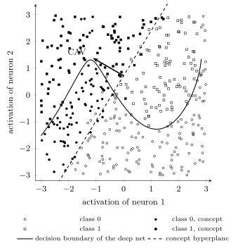
B-cavFig. 1 draws the CAV of the heat-wave
concept for a deep net with two hidden layers of 16
neurons, trained on the daily weather at Krems an der Donau
of the training years 2000–2018 and tested on 2019–2024. A
data point is a window of five days, its feature vector
holds the daily maximum and minimum temperature and the rain amount
of each day, and its label says whether at least 1 mm of
rain fell on the sixth day. The concept is specified by 40 heat
waves, windows with a daily maximum of at least
$30\,^{\circ}$C on all five days, and 40 windows that are not,
drawn from the 9127 windows of the record. The plane drawn passes
through the mean activation of the first hidden layer
and is spanned by the CAV and the direction orthogonal to it
along which the activations vary most. The concept
hyperplane therefore meets the plane in a vertical line, and
the CAV is its horizontal axis. Two classification problems appear in the figure. The first is the concept classification that $g(\vz)$ solves on the activations. The second is the task the deep net is trained for, whose decision boundary on the plane is the solid line: rain is predicted to its right, where every heat wave lies. Training $g(\vz)$ on all 9127 windows instead turns the CAV by 26 degrees.
pythondemos/cav.py
Write the trained deep net as a concatenation of two functions, the activations $\vz = f(\featurevec)$ of the chosen hidden layer and a score $s(\vz)$ that the remaining layers assign to one label. The conceptual sensitivity of a data point is the directional derivative of that score along the unit CAV $\vv \defeq \widehat{\weights} / \norm{\widehat{\weights}}$, which for differentiable $s$ equals the inner product of the gradient of $s$ with $\vv$ (Rudin, 1976, Example 9.18), \begin{equation} \label{equ_cav_sensitivity} S(\featurevec) \defeq \innerprod{\nabla s\big(f(\featurevec)\big)}{\vv} \text{.} \end{equation} It measures how much the score for that label moves when the activations move a little towards the concept (Kim et al., 2018, Sect. 3.3). The orientation convention gives the sign its meaning: $S(\featurevec) > 0$ says the score rises towards the concept, and the opposite normal vector would flip every sensitivity.
B-tcavThe sensitivity $S(\featurevec)$ delivers one number per data point. TCAV collects these numbers over one label: the TCAV score is the fraction of the data points carrying that label for which $S(\featurevec) > 0$ (Kim et al., 2018, Sect. 3.4). A random set of non-concept data points also yields a CAV, so a single such fraction is not evidence alone. A random concept is a set of data points drawn at random and labelled as if they carried a concept. It is as likely to raise the score as to lower it, so its TCAV score, the fraction of positive sensitivities, is one half on average. The CAV is therefore refitted against many fresh draws of non-concept data points, and the resulting TCAV scores are compared with those of random concepts: a concept the deep net responds to scores consistently away from one half, a random one does not (Kim et al., 2018, Sect. 3.5). The explanation delivered is a single number attached to a concept, a label and a layer. Unlike the sensitivity $S(\featurevec)$, which is defined for a single data point, it describes a whole class of data points rather than a single prediction (Kim et al., 2018, Sect. 2.1). For the deep net of Fig. 1, moving along the heat-wave CAV raises the rain score at every test window followed by rain, and moving along the CAV of a cold wave, five days with a minimum of at most $-5\,^{\circ}$C, lowers it at every one of them. The record agrees: rain follows 30% of the heat waves and 16% of the cold waves, against 23% of all windows. Random concepts score one half on average.
Training the linear classifier $g(\vz)$ and evaluating the sensitivity $S(\featurevec)$ both read quantities inside the deep net: the activations $f(\featurevec)$ of the chosen layer, and the gradient $\nabla s(\vz)$ of the score with respect to them. A CAV is therefore unavailable for a system that returns predictions for submitted feature vectors and nothing else, such as a deep net served behind an interface or supplied by a vendor. An explanation produced by local interpretable model-agnostic explanations (LIME), by contrast, needs predictions and nothing else: its local approximation is fitted to predictions obtained by querying the learned hypothesis $\learnthypothesis$ (Ribeiro et al., 2016, Sect. 3). A second consequence of reading the internals is that a CAV is not a property of $\learnthypothesis$ alone: the split into $f$ and $s$ is a choice of layer, and two deep nets that deliver the same $\learnthypothesis$ through different layers have different CAVs.
Both functions a CAV involves are defined on the space of activations: $g(\vz)$ approximates concept membership there, and the sensitivity $S(\featurevec)$ is a directional derivative of the score $s$ on that same space. A CAV therefore concerns the interpretability of the deep net rather than its explainability; mechanistic interpretability studies such directions.
See also: deep net, feature, linear classifier, trustworthy artificial intelligence, interpretability, mechanistic interpretability, transparency, explanation, explainability, neuron, decision boundary, hyperplane, local interpretable model-agnostic explanations.
@misc{dictml_cav,
  author = {Jung, Alexander},
  editor = {Olioumtsevits, Konstantina and Schnoor, Ekkehard},
  title = {concept activation vector (CAV)},
  howpublished = {Dictionary of Applied Machine Learning (course edition)},
  year = {2026},
  doi = {10.5281/zenodo.21569296},
  note = {ISBN 978-952-64-3013-3, CC BY 4.0, retrieved 2026-10-06},
  url = {https://dictionaryofml.org/terms/cav.html}
}