B-fig writes when the script runsDictionary of Applied Machine Learning · concept activation vector (CAV)
Numerical companion to the entry concept activation vector (CAV): it recomputes what the entry states and prints one line per check
A CAV is fitted the way the entry describes it, on real data. The data points are five consecutive days of weather at Krems an der Donau (GeoSphere Austria, station 3805, 2000-2024): the daily maximum and minimum temperature and the rain of each day, fifteen numbers, and the label says whether at least 1 mm of rain fell on the sixth day. A small deep net (15 -> 16 -> 16 -> 1) predicts that label; the first hidden layer, sixteen neurons, is the layer whose activations the CAV lives in.
Run it without installing anything:uv run https://dictionaryofml.org/terms/cav.py
uv downloads this script and the pinned NumPy and Matplotlib it needs, then runs it; the script fetches any input file it uses. To keep the output files, download cav.py into a folder and run uv run cav.py there. With NumPy and Matplotlib already installed, python3 cav.py, from any directory — it writes its output files into the current directory. Fixed seeds, so the printed numbers reproduce exactly. Download cav.py · Notebook · Open in Colab
One cell per block of the script: the code, and what that code printed when it last ran here
"""
cav.py — numerical companion to the glossary entry 'concept activation
vector (CAV)'.

Purpose
-------
A CAV is fitted the way the entry describes it, on real data.  The data
points are five consecutive days of weather at Krems an der Donau
(GeoSphere Austria, station 3805, 2000-2024): the daily maximum and minimum
temperature and the rain of each day, fifteen numbers, and the label says
whether at least 1 mm of rain fell on the sixth day.  A small deep net
(15 -> 16 -> 16 -> 1) predicts that label; the first hidden layer, sixteen
neurons, is the layer whose activations the CAV lives in.

The concept is a heat wave: five days in a row with a maximum of at least
30 degrees.  It is not a feature the net was built with, and it is
specified by examples: windows that are heat waves and windows that are
not.  A linear classifier fitted to the activations of those examples
separates them by a hyperplane; its normal vector is the CAV.  Testing with
CAVs asks whether the net's rain score rises when the activations move a
little along the CAV, at the windows followed by rain.  A cold wave (five
days with a minimum of at most -5 degrees) is fitted the same way.  Both
concepts turn out to be ones the net uses, in opposite directions, and the
record says why: rain follows a heat wave more often than an average
window (30% against 23%) and a cold wave less often (16%).  The control the method rests on is
the random concept, a set of windows drawn at random and labelled as if
they carried a concept, whose TCAV score sits near one half.

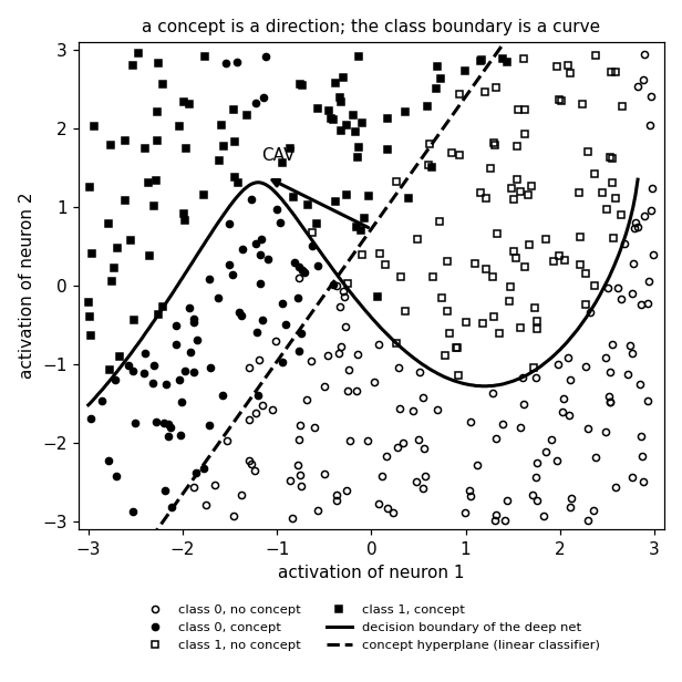
The figure draws a plane a reader can look at: through the mean activation,
spanned by the CAV and the leading direction of the activations orthogonal
to it.  In that plane the concept hyperplane is a vertical line and the
CAV the horizontal axis, so the separation the classifier found is visible
as it is; the net's decision boundary, the curve where its score on that
plane crosses the base-rate threshold, is what the rain score does across
it.  A first version used a two-neuron layer so that the activations
themselves formed a plane; there every direction was either along the
score's gradient or against it, random concepts scored 0 or 1 and the
control was worthless.  Sixteen neurons restore it.

Self-contained (numpy + matplotlib, urllib for the download), fixed seed.

Blocks
------
[B-fetch]  25 years of daily tmin, tmax and rain at Krems, downloaded from
           the GeoSphere data hub and written to cav_weather.csv; five-day
           windows and their sixth-day rain labels.
[B-net]    A deep net 15 -> 16 -> 16 -> 1 (ReLU, logistic output) trained
           with Adam on 2000-2018 and tested on 2019-2024; it beats
           always answering the base rate on the held-out years.  Rain is predicted
           when the score exceeds the base rate.
[B-cav]    The CAV: a binary linear classifier separating heat-wave windows
           from non-heat-wave windows by their sixteen activations, fitted
           to forty examples of each kind, all of which the figure draws.
           Its weight vector, the CAV, is the normal of the separating
           hyperplane; the same fit on every window of the record gives a
           nearby direction.
[B-tcav]   Conceptual sensitivity: the directional derivative of the rain
           score along the unit CAV at the test windows followed by rain,
           and the TCAV score, the fraction of them where it is positive.
           The CAV is refitted against fresh draws of non-concept windows,
           and random "concepts" (windows drawn at random as positives)
           are scored the same way: their scores are coin flips between 0
           and 1 with mean one half, since the score's gradient points the
           same way at nearly every rainy window, and a concept counts
           when its refits agree (the original method's two-sided test).
           The cold wave is scored the same way.
[B-fig]    The figure: the plane through the mean activation spanned by
           the CAV and the leading orthogonal direction; the test windows,
           the eighty examples and the concept hyperplane projected onto
           it, and the net's boundary on it.  Written to
           cav_points.csv, cav_windows.csv, cav_boundary.csv,
           cav_cavline.csv, cav_arrow.csv and cav.png.

Outputs
-------
cav_weather.csv  : date, tmin, tmax, rr for every day downloaded
cav_points.csv   : z1, z2, concept, grp for the eighty concept examples
                   (plane coordinates: z1 along the CAV)
cav_windows.csv  : z1, z2, rain for a sample of test windows
cav_boundary.csv : the net's decision boundary on the plane
cav_cavline.csv  : the concept hyperplane
cav_arrow.csv    : the CAV, drawn from a point on the hyperplane
cav.png          : preview (checking only)
"""

import json
import urllib.request
from pathlib import Path

import numpy as np
import matplotlib

OUT_DIR = Path(__file__).parent

matplotlib.use("Agg")
import matplotlib.pyplot as plt

report = []                         # collects (check name, pass/fail) pairs


def check(name, ok):                # records and prints one verification
    report.append((name, bool(ok)))
    print(f"  [{'ok' if ok else 'FAIL'}] {name}")


rng = np.random.default_rng(20260917)
DAYS = 5                            # a data point is this many days in a row
HOT, COLD = 30.0, -5.0              # heat wave: tmax >= HOT on all days;
                                    # cold wave: tmin <= COLD on all days
WET = 1.0                           # mm on the sixth day counting as rain
NEX = 40                            # concept examples of each kind, all drawn
25 years of daily tmin, tmax and rain at Krems, downloaded from the GeoSphere data hub and written to cav_weather.csv; five-day windows and their sixth-day rain labels.
URL = ("https://dataset.api.hub.geosphere.at/v1/station/historical/"
       "klima-v2-1d?parameters=tlmin,tlmax,rr&station_ids=3805"
       "&start=2000-01-01&end=2024-12-31")
with urllib.request.urlopen(URL, timeout=180) as resp:
    payload = json.load(resp)
params = payload["features"][0]["properties"]["parameters"]
stamps = [t[:10] for t in payload["timestamps"]]
tmin = np.array([np.nan if v is None else v for v in params["tlmin"]["data"]])
tmax = np.array([np.nan if v is None else v for v in params["tlmax"]["data"]])
rain = np.array([np.nan if v is None else v for v in params["rr"]["data"]])
with open(OUT_DIR / "cav_weather.csv", "w") as fh:
    fh.write("date,tmin,tmax,rr\n")
    for d, lo, hi, r in zip(stamps, tmin, tmax, rain):
        fh.write(f"{d},{lo},{hi},{r}\n")
check(f"[B-fetch] {len(stamps)} days downloaded, 2000-2024",
      len(stamps) > 9000 and stamps[0] == "2000-01-01")

# five-day windows: features are the five maxima, the five minima and the
# five rain amounts (log-scaled); the label is rain on the day after
n = len(stamps) - DAYS
X = np.stack([np.stack([tmax[i:i + DAYS], tmin[i:i + DAYS],
                        np.log1p(np.maximum(rain[i:i + DAYS], 0.0))]).ravel()
              for i in range(n)])
y = (rain[DAYS:DAYS + n] >= WET).astype(float)
year = np.array([int(stamps[i + DAYS][:4]) for i in range(n)])
ok_rows = ~np.isnan(X).any(axis=1) & ~np.isnan(rain[DAYS:DAYS + n])
X, y, year, win_start = X[ok_rows], y[ok_rows], year[ok_rows], np.arange(n)[ok_rows]
heat = (X[:, :DAYS] >= HOT).all(axis=1)
cold = (X[:, DAYS:2 * DAYS] <= COLD).all(axis=1)
print(f"  {len(y)} windows of {DAYS} days; rain follows {y.mean():.0%} of them; "
      f"{heat.sum()} heat waves, {cold.sum()} cold waves")
check("[B-fetch] both concepts occur often enough to supply examples",
      heat.sum() >= 2 * NEX and cold.sum() >= 2 * NEX)

tr, te = year <= 2018, year >= 2019
mu, sd = X[tr].mean(axis=0), X[tr].std(axis=0)
Xs = (X - mu) / sd
  [ok] [B-fetch] 9132 days downloaded, 2000-2024
  9127 windows of 5 days; rain follows 23% of them; 112 heat waves, 87 cold waves
  [ok] [B-fetch] both concepts occur often enough to supply examples
  loss 0.634 -> 0.493; test log-loss 0.529 against 0.553 for always answering the base rate; at the base-rate threshold the net predicts rain for 56% of the rainy test days and is right on 63% of all test days
A deep net 15 -> 16 -> 16 -> 1 (ReLU, logistic output) trained with Adam on 2000-2018 and tested on 2019-2024; it beats always answering the base rate on the held-out years. Rain is predicted when the score exceeds the base rate.
H1, H2 = 16, 16


relu = lambda a: np.maximum(a, 0.0)


def forward(Xin, P):
    W1, b1, W2, b2, w3, c = P
    Z = relu(Xin @ W1 + b1)                         # the chosen layer (n, 16)
    Hh = relu(Z @ W2 + b2)
    return Z, Hh, Hh @ w3 + c                       # score: larger, rain likelier


def score_from_plane(Z, P):
    """The rest of the net, s(z): from the chosen layer's activations to the
    score."""
    _, _, W2, b2, w3, c = P
    return relu(Z @ W2 + b2) @ w3 + c


P = [rng.normal(0, np.sqrt(2 / X.shape[1]), (X.shape[1], H1)), np.zeros(H1),
     rng.normal(0, np.sqrt(2 / H1), (H1, H2)), np.zeros(H2),
     rng.normal(0, 0.3, H2), 0.0]
WD = 3e-3                                           # weight decay
# Adam (Kingma and Ba, 2015): plain gradient descent with a small step
# left this net answering the base rate everywhere
m1 = [np.zeros_like(np.asarray(q, dtype=float)) for q in P]
m2 = [np.zeros_like(np.asarray(q, dtype=float)) for q in P]
lrate, losses = 0.01, []
Xtr, ytr = Xs[tr], y[tr]
for step in range(1500):
    Z, Hh, s = forward(Xtr, P)
    p = 1.0 / (1.0 + np.exp(-s))
    losses.append(float(-np.mean(ytr * np.log(p + 1e-9)
                                 + (1 - ytr) * np.log(1 - p + 1e-9))))
    err = (p - ytr) / len(ytr)                      # d loss / d score
    W1, b1, W2, b2, w3, c = P
    g_w3, g_c = Hh.T @ err + WD * w3, err.sum()
    dH = np.outer(err, w3) * (Hh > 0)
    g_W2, g_b2 = Z.T @ dH + WD * W2, dH.sum(axis=0)
    dZ = (dH @ W2.T) * (Z > 0)
    g_W1, g_b1 = Xtr.T @ dZ + WD * W1, dZ.sum(axis=0)
    grads = [g_W1, g_b1, g_W2, g_b2, g_w3, g_c]
    newP = []
    for k, (q, g) in enumerate(zip(P, grads)):
        m1[k] = 0.9 * m1[k] + 0.1 * g
        m2[k] = 0.999 * m2[k] + 0.001 * g * g
        mh = m1[k] / (1 - 0.9 ** (step + 1))
        vh = m2[k] / (1 - 0.999 ** (step + 1))
        newP.append(q - lrate * mh / (np.sqrt(vh) + 1e-8))
    P = newP

Zall, _, sall = forward(Xs, P)
pall = 1.0 / (1.0 + np.exp(-sall))
# the net's decision rule: predict rain when the score exceeds the base
# rate of the years it was fitted to (a score above THR)
THR = float(np.log(y[tr].mean() / (1 - y[tr].mean())))
ll = lambda m: float(-np.mean(y[m] * np.log(pall[m] + 1e-9)
                              + (1 - y[m]) * np.log(1 - pall[m] + 1e-9)))
ll_const = float(-np.mean(y[te] * np.log(y[tr].mean())
                          + (1 - y[te]) * np.log(1 - y[tr].mean())))  # the base-rate rule
acc_te = float(((sall[te] > THR) == (y[te] > 0.5)).mean())
hit = float((sall[te][y[te] > 0.5] > THR).mean())
print(f"  loss {losses[0]:.3f} -> {losses[-1]:.3f}; test log-loss {ll(te):.3f} "
      f"against {ll_const:.3f} for always answering the base rate; at the "
      f"base-rate threshold the net predicts rain for {hit:.0%} of the rainy "
      f"test days and is right on {acc_te:.0%} of all test days")
check("[B-net] the net beats always answering the base rate on the held-out years",
      ll(te) < ll_const - 0.01)


def fit_linear(Xin, yin, steps=2000, lr=0.3, l2=1e-2):
    """Logistic regression by gradient descent, with a small ridge penalty
    so that separable examples still fix a direction; returns (w, b)."""
    w, b = np.zeros(Xin.shape[1]), 0.0
    for _ in range(steps):
        p = 1.0 / (1.0 + np.exp(-(Xin @ w + b)))
        w -= lr * (Xin.T @ (p - yin) / len(yin) + l2 * w)
        b -= lr * (p - yin).mean()
    return w, b


acc = lambda w, b, Xin, yin: float((((Xin @ w + b) > 0) == (yin > 0.5)).mean())

# what the record itself says about the two concepts
after_heat, after_cold = float(y[heat].mean()), float(y[cold].mean())
print(f"  rain follows {after_heat:.0%} of the heat waves and {after_cold:.0%} "
      f"of the cold waves, against {y.mean():.0%} of all windows")
check("[B-net] the record says rain follows a heat wave more often than "
      "an average window", after_heat > y.mean() + 0.05)
check("[B-net] ... and a cold wave less often", after_cold < y.mean() - 0.05)
  [ok] [B-net] the net beats always answering the base rate on the held-out years
  rain follows 30% of the heat waves and 16% of the cold waves, against 23% of all windows
  [ok] [B-net] the record says rain follows a heat wave more often than an average window
  [ok] [B-net] ... and a cold wave less often
  the CAV is fitted to 80 examples, 40 of them heat waves; it points along (-0.08, 0.57)
  the fitted hyperplane separates 75 of the 80 examples
The CAV: a binary linear classifier separating heat-wave windows from non-heat-wave windows by their sixteen activations, fitted to forty examples of each kind, all of which the figure draws. Its weight vector, the CAV, is the normal of the separating hyperplane; the same fit on every window of the record gives a nearby direction.
def examples(concept, n=NEX):
    """n concept windows and n non-concept windows, drawn at random from
    the record: the examples a user would supply, not a curated selection."""
    pos = rng.choice(np.where(concept)[0], n, replace=False)
    neg = rng.choice(np.where(~concept)[0], n, replace=False)
    idx = np.concatenate([pos, neg])
    return idx, np.concatenate([np.ones(n), np.zeros(n)])


idx_ex, y_ex = examples(heat)
Z_ex = Zall[idx_ex]
w_cav, b_cav = fit_linear(Z_ex, y_ex)
cav = w_cav / np.linalg.norm(w_cav)                 # the CAV, unit length
print(f"  the CAV is fitted to {len(idx_ex)} examples, {int(y_ex.sum())} of "
      f"them heat waves; it points along ({cav[0]:.2f}, {cav[1]:.2f})")
n_sep = int(round(acc(w_cav, b_cav, Z_ex, y_ex) * len(y_ex)))
print(f"  the fitted hyperplane separates {n_sep} of the {len(y_ex)} examples")
check("[B-cav] the fitted hyperplane separates nearly all eighty examples",
      n_sep >= 0.85 * len(y_ex))
# ten examples of each kind fix the direction: the same fit on every window
# of the record is the reference
w_pool, _ = fit_linear(Zall, heat.astype(float))
cos_pool = float(cav @ (w_pool / np.linalg.norm(w_pool)))
print(f"  the same fit on all {len(y)} windows gives a direction "
      f"{np.degrees(np.arccos(min(cos_pool, 1.0))):.0f} degrees away")
check("[B-cav] forty examples of each kind fix a direction near the record's",
      cos_pool > 0.8)

idx_cold, y_cold = examples(cold)
w_cc, b_cc = fit_linear(Zall[idx_cold], y_cold)
cav_cold = w_cc / np.linalg.norm(w_cc)
  [ok] [B-cav] the fitted hyperplane separates nearly all eighty examples
  the same fit on all 9127 windows gives a direction 26 degrees away
  [ok] [B-cav] forty examples of each kind fix a direction near the record's
  moving along the heat-wave CAV raises the rain score at 100% of the 528 rainy test windows, along the cold-wave CAV at 0%
  over 100 refits with fresh non-concept draws the heat-wave TCAV score is 0.99 +- 0.10; random concepts give 0.58 +- 0.49
  99% of the heat-wave refits score above one half; Welch t-statistic against the random concepts 8.1
Conceptual sensitivity: the directional derivative of the rain score along the unit CAV at the test windows followed by rain, and the TCAV score, the fraction of them where it is positive. The CAV is refitted against fresh draws of non-concept windows, and random "concepts" (windows drawn at random as positives) are scored the same way: their scores are coin flips between 0 and 1 with mean one half, since the score's gradient points the same way at nearly every rainy window, and a concept counts when its refits agree (the original method's two-sided test). The cold wave is scored the same way.
EPS = 1e-4


def sensitivity(direction, Zpts):
    """Directional derivative of the rain score along the unit direction."""
    d = direction / np.linalg.norm(direction)
    return (score_from_plane(Zpts + EPS * d, P) - score_from_plane(Zpts, P)) / EPS


rainy = te & (y > 0.5)                              # test windows followed by rain
Zr = Zall[rainy]
tcav = lambda v: float((sensitivity(v, Zr) > 0).mean())
tcav_heat, tcav_cold = tcav(cav), tcav(cav_cold)
print(f"  moving along the heat-wave CAV raises the rain score at "
      f"{tcav_heat:.0%} of the {len(Zr)} rainy test windows, along the "
      f"cold-wave CAV at {tcav_cold:.0%}")

# does the choice of non-concept examples move the score?  and the random-
# concept reference (the original method's statistical test)
REFITS = 100
scores_heat, scores_rand = [], []
for _ in range(REFITS):
    i, yy = examples(heat)
    w, _ = fit_linear(Zall[i], yy)
    scores_heat.append(tcav(w))
    i = rng.choice(len(y), 2 * NEX, replace=False)   # a random "concept"
    w, _ = fit_linear(Zall[i], yy)
    scores_rand.append(tcav(w))
scores_heat, scores_rand = np.array(scores_heat), np.array(scores_rand)
print(f"  over {REFITS} refits with fresh non-concept draws the heat-wave TCAV "
      f"score is {scores_heat.mean():.2f} +- {scores_heat.std():.2f}; random "
      f"concepts give {scores_rand.mean():.2f} +- {scores_rand.std():.2f}")
# The score's gradient points the same way at nearly every rainy window
# (the net is close to one-dimensional in its activations), so a direction
# either raises the score at almost all of them or at almost none: the
# scores of random concepts are coin flips between 0 and 1 with mean one
# half, and a concept counts when its refits agree, as the two-sided test
# of the original method asks
agree = float((scores_heat > 0.5).mean())
t_stat = ((scores_heat.mean() - scores_rand.mean())
          / np.sqrt(scores_heat.var() / REFITS + scores_rand.var() / REFITS))
print(f"  {agree:.0%} of the heat-wave refits score above one half; "
      f"Welch t-statistic against the random concepts {t_stat:.1f}")
check("[B-tcav] the heat-wave TCAV score is far above one half",
      scores_heat.mean() > 0.75)
check("[B-tcav] the cold-wave score lies on the other side of one half",
      tcav_cold < 0.25)
check("[B-tcav] random concepts score one half on average",
      abs(scores_rand.mean() - 0.5) < 0.15)
check("[B-tcav] the heat-wave refits agree, unlike the coin flips",
      agree >= 0.8 and t_stat > 4)
  [ok] [B-tcav] the heat-wave TCAV score is far above one half
  [ok] [B-tcav] the cold-wave score lies on the other side of one half
  [ok] [B-tcav] random concepts score one half on average
  [ok] [B-tcav] the heat-wave refits agree, unlike the coin flips
The figure: the plane through the mean activation spanned by the CAV and the leading orthogonal direction; the test windows, the eighty examples and the concept hyperplane projected onto it, and the net's boundary on it. Written to cav_points.csv, cav_windows.csv, cav_boundary.csv, cav_cavline.csv, cav_arrow.csv and cav.png.
# The plane: through the mean activation, spanned by the unit CAV (first
# axis) and the leading principal direction of the activations after their
# CAV component is removed (second axis). Plane coordinates of a point z:
# a = cav . (z - zbar), b = u2 . (z - zbar).
zbar = Zall[te].mean(axis=0)
resid = (Zall[te] - zbar) - np.outer((Zall[te] - zbar) @ cav, cav)
_, _, vt = np.linalg.svd(resid, full_matrices=False)
u2 = vt[0]
to_plane = lambda Zin: np.stack([(Zin - zbar) @ cav, (Zin - zbar) @ u2], 1)
from_plane = lambda a, b: zbar + np.outer(a, cav) + np.outer(b, u2)

Q_ex = to_plane(Z_ex)
with open(OUT_DIR / "cav_points.csv", "w") as fh:
    fh.write("z1,z2,concept,grp\n")
    for (a, b), k in zip(Q_ex, y_ex):
        fh.write(f"{a:.4f},{b:.4f},{int(k)},k{int(k)}\n")
sample = rng.choice(np.where(te)[0], 400, replace=False)
Q_win = to_plane(Zall[sample])
with open(OUT_DIR / "cav_windows.csv", "w") as fh:
    fh.write("z1,z2,rain\n")
    for (a, b), i in zip(Q_win, sample):
        fh.write(f"{a:.4f},{b:.4f},{int(y[i])}\n")
lo, hi = Q_win.min(axis=0) - 0.2, Q_win.max(axis=0) + 0.2

# the net's boundary on the plane: for each a, the b where the score on the
# plane crosses the base-rate threshold
grid_a, grid_b = np.linspace(lo[0], hi[0], 161), np.linspace(lo[1], hi[1], 801)
with open(OUT_DIR / "cav_boundary.csv", "w") as fh:
    fh.write("z1,z2\n")
    for a in grid_a:
        sc = score_from_plane(from_plane(np.full_like(grid_b, a), grid_b), P) - THR
        sign = np.where(np.diff(np.sign(sc)))[0]
        if len(sign):
            fh.write(f"{a:.4f},{grid_b[sign[0]]:.4f}\n")
bnd = np.loadtxt(OUT_DIR / "cav_boundary.csv", delimiter=",", skiprows=1, ndmin=2)
check("[B-fig] the net's boundary crosses the plane", len(bnd) > 20)

# the concept hyperplane w . z + b = 0 meets the plane in the vertical line
# a = a0 (its normal IS the first axis); the CAV is drawn from that line
a0 = float(-(b_cav + w_cav @ zbar) / np.linalg.norm(w_cav))
with open(OUT_DIR / "cav_cavline.csv", "w") as fh:
    fh.write("z1,z2\n")
    fh.write(f"{a0:.4f},{lo[1]:.4f}\n{a0:.4f},{hi[1]:.4f}\n")
foot = np.array([a0, 0.5 * (lo[1] + hi[1])])
ARROW = 0.25 * (hi[0] - lo[0])
with open(OUT_DIR / "cav_arrow.csv", "w") as fh:
    fh.write("z1,z2\n")
    fh.write(f"{foot[0]:.4f},{foot[1]:.4f}\n")
    fh.write(f"{foot[0] + ARROW:.4f},{foot[1]:.4f}\n")
print("  wrote cav_points.csv, cav_windows.csv, cav_boundary.csv, "
      "cav_cavline.csv, cav_arrow.csv")

fig, ax = plt.subplots(figsize=(5.8, 5.8))
ax.plot(Q_win[:, 0], Q_win[:, 1], ".", ms=3, color="0.6", label="test window")
ax.plot(bnd[:, 0], bnd[:, 1], "k-", lw=2.0,
        label="decision boundary of the deep net")
ax.plot([a0, a0], [lo[1], hi[1]], "k--", lw=2.0,
        label="concept hyperplane (linear classifier)")
for k, fill, lbl in ((1, "k", "heat-wave example"),
                     (0, "none", "non-heat-wave example")):
    sel = y_ex == k
    ax.plot(Q_ex[sel, 0], Q_ex[sel, 1], "o", ms=8, mfc=fill, mec="k", lw=0,
            label=lbl)
ax.annotate("", xy=(foot[0] + ARROW, foot[1]), xytext=foot,
            arrowprops=dict(arrowstyle="-|>", lw=2.0, color="k"))
ax.annotate("CAV", (foot[0] + ARROW + 0.02 * (hi[0] - lo[0]), foot[1]),
            fontsize=10, va="center")
ax.set_xlim(lo[0], hi[0])
ax.set_ylim(lo[1], hi[1])
ax.set_xlabel("activation along the CAV")
ax.set_ylabel("activation along the leading orthogonal direction")
ax.set_title("a concept is a direction in the activations of a hidden layer",
             fontsize=10)
ax.legend(frameon=False, fontsize=7.5, loc="upper center",
          bbox_to_anchor=(0.5, -0.13), ncol=2)
fig.tight_layout()
fig.savefig(OUT_DIR / "cav.png", dpi=110)
print(f"  wrote {OUT_DIR / 'cav.png'}")

bad = [n for n, ok in report if not ok]
print(f"\n{len(report) - len(bad)}/{len(report)} checks passed"
      + (f"; FAILED: {bad}" if bad else ""))
  [ok] [B-fig] the net's boundary crosses the plane
  wrote cav_points.csv, cav_windows.csv, cav_boundary.csv, cav_cavline.csv, cav_arrow.csv
  wrote /Users/junga1/dictionaryappliedml/pythondemos/cav.png

12/12 checks passed
B-fig writes when the script runs