P-vector writes when the script runsDictionary of Applied Machine Learning · variance
Numerical companion to the entry variance: it recomputes what the entry states and prints one line per check
One block per paragraph of the entry (marked [P...]): each block verifies numerically what the corresponding statement asserts. Self-contained (numpy/matplotlib only), fixed seed.
Run it without installing anything:uv run https://dictionaryofml.org/terms/variance.py
uv downloads this script and the pinned NumPy and Matplotlib it needs, then runs it; the script fetches any input file it uses. To keep the output files, download variance.py into a folder and run uv run variance.py there. With NumPy and Matplotlib already installed, python3 variance.py, from any directory — it writes its output files into the current directory. Fixed seeds, so the printed numbers reproduce exactly. Download variance.py · Notebook · Open in Colab
One cell per block of the script: the code, and what that code printed when it last ran here
"""
variance.py — numerical companion to the glossary entry 'variance'.

One block per paragraph of the entry (marked [P...]): each block verifies
numerically what the corresponding statement asserts. Self-contained
(numpy/matplotlib only), fixed seed.

Blocks
------
[P-def]    The variance of a real-valued RV y (such as the numeric label
           of a data point) is E{(y - E{y})^2}: the empirical variance of
           realizations of i.i.d. RVs with variance sigma^2 matches
           sigma^2, and shifting
           the RV leaves the variance unchanged (it measures spread
           around the mean, not location). The entry's figure shows seven
           measured daily maximum temperatures (see Data below): their
           sample mean is exactly 20.5 degC, their sample variance
           6.34/7, and the figure data is written to
           variance_weather.csv. A dataset D of labels defines a
           discrete RV y~ = y^(I) with I uniform on {1, ..., m}; the
           variance of y~, computed from that uniform pmf, is the sample
           variance of D (average squared deviation from the sample
           mean).
[P-min]    The variance is the minimum of the risk E{(y - b)^2} over
           constants b, attained at b = E{y} (grid search).
[P-erm]    The simplest ML problem: predict the label y without any
           features. The hypothesis space consists of the constant maps
           h(.) = b (a single bias term). ERM with the squared error
           loss on the training set of measured temperatures amounts to
           finding the constant that best predicts a label: the grid
           minimizer of the training error is the sample mean 20.5 degC
           (the dashed line of the entry's figure), the training error
           of that learned hypothesis is the sample variance of the
           labels, and at the population level every constant prediction
           has risk >= variance — the baseline.
[P-vector] For a random vector, E{||x - E{x}||^2} equals trace(C), the
           sum of the per-entry variances (checked against the analytic
           covariance matrix C = A A^T and against np.cov).

Outputs
-------
variance_weather.csv : figure data for the entry's pgfplots figure
                       (day, tmax, mean, dev).
variance.png         : preview figure (checking only).

Data
----
Daily maximum temperatures (tmax), Helsinki Kaisaniemi weather station,
24-30 August 2026, from the Finnish Meteorological Institute's open
data service (https://opendata.fmi.fi, stored query
fmi::observations::weather::daily::simple), retrieved 2026-09-01.

Data generated by pythondemos/variance.py.
"""

import numpy as np
import matplotlib

matplotlib.use("Agg")
import matplotlib.pyplot as plt
from pathlib import Path

OUT_DIR = Path(__file__).parent

rng = np.random.default_rng(42)
report = []


def check(name, ok):
    report.append((name, bool(ok)))
    print(f"  [{'ok' if ok else 'FAIL'}] {name}")
The variance of a real-valued RV y (such as the numeric label of a data point) is E{(y - E{y})^2}: the empirical variance of realizations of i.i.d. RVs with variance sigma^2 matches sigma^2, and shifting the RV leaves the variance unchanged (it measures spread around the mean, not location). The entry's figure shows seven measured daily maximum temperatures (see Data below): their sample mean is exactly 20.5 degC, their sample variance 6.34/7, and the figure data is written to variance_weather.csv. A dataset D of labels defines a discrete RV y~ = y^(I) with I uniform on {1, ..., m}; the variance of y~, computed from that uniform pmf, is the sample variance of D (average squared deviation from the sample mean).
print("[P-def] variance = E{(y - E y)^2}; sample variance = variance of "
      "the dataset-induced discrete RV")
sigma = 1.7
m = 10**6
y = sigma * rng.standard_normal(m)
var_emp = np.mean((y - y.mean()) ** 2)
check("empirical variance matches sigma^2 = 2.89",
      abs(var_emp - sigma**2) < 2e-2)
check("shifting by +5 leaves the variance unchanged",
      abs(np.mean(((y + 5) - (y + 5).mean()) ** 2) - var_emp) < 1e-9)
scales = [0.5, 1.0, 2.0]
vars_scaled = [np.mean(((s * y) - (s * y).mean()) ** 2) for s in scales]
check("scaling by s multiplies the variance by s^2",
      all(abs(v - s**2 * var_emp) < 1e-6 * max(1, s**2 * var_emp)
          for s, v in zip(scales, vars_scaled)))
# daily max temperatures y^(1), ..., y^(7), Helsinki Kaisaniemi,
# 24-30 August 2026 (FMI open data; see the Data section above)
d = np.array([20.1, 19.9, 22.2, 21.7, 20.3, 19.6, 19.7])
days = np.arange(1, d.size + 1)
check("sample mean of the measured temperatures is 20.5 degC",
      np.isclose(d.mean(), 20.5))
check("their sample variance is 6.34/7",
      np.isclose(np.mean((d - d.mean()) ** 2), 6.34 / 7))
rows = np.column_stack([days, d, np.full(d.size, d.mean()), d - d.mean()])
np.savetxt(OUT_DIR / "variance_weather.csv", rows,
           fmt=["%d", "%.1f", "%.4f", "%.4f"], delimiter=",",
           header="day,tmax,mean,dev", comments="")
p = np.full(d.size, 1 / d.size)               # uniform pmf of y~ = y^(I)
mean_discrete = np.sum(p * d)
var_discrete = np.sum(p * (d - mean_discrete) ** 2)
sample_var = np.mean((d - d.mean()) ** 2)
check("pmf-based variance of y~ equals the sample variance",
      np.isclose(var_discrete, sample_var))
check("matches np.var (ddof=0)", np.isclose(sample_var, np.var(d)))
[P-def] variance = E{(y - E y)^2}; sample variance = variance of the dataset-induced discrete RV
  [ok] empirical variance matches sigma^2 = 2.89
  [ok] shifting by +5 leaves the variance unchanged
  [ok] scaling by s multiplies the variance by s^2
  [ok] sample mean of the measured temperatures is 20.5 degC
  [ok] their sample variance is 6.34/7
  [ok] pmf-based variance of y~ equals the sample variance
  [ok] matches np.var (ddof=0)
The variance is the minimum of the risk E{(y - b)^2} over constants b, attained at b = E{y} (grid search).
print("[P-min] variance = min over constants b of E{(y - b)^2}")
ys = y[:100_000]                               # draws from [P-def]
b_grid = np.linspace(-3, 3, 601)
risk = np.array([np.mean((ys - b) ** 2) for b in b_grid])
var_ys = np.mean((ys - ys.mean()) ** 2)
check("risk is minimized at the mean (grid resolution 0.01)",
      abs(b_grid[np.argmin(risk)] - ys.mean()) < 0.02)
check("minimum of the risk equals the variance",
      abs(risk.min() - var_ys) < 1e-3)
[P-min] variance = min over constants b of E{(y - b)^2}
  [ok] risk is minimized at the mean (grid resolution 0.01)
  [ok] minimum of the risk equals the variance
The simplest ML problem: predict the label y without any features. The hypothesis space consists of the constant maps h(.) = b (a single bias term). ERM with the squared error loss on the training set of measured temperatures amounts to finding the constant that best predicts a label: the grid minimizer of the training error is the sample mean 20.5 degC (the dashed line of the entry's figure), the training error of that learned hypothesis is the sample variance of the labels, and at the population level every constant prediction has risk >= variance — the baseline.
print("[P-erm] ERM over the constant maps h(.) = b: the learned bias "
      "term is the sample mean; the variance is the baseline")
y_train = d                                    # temperatures as labels
b_train_grid = np.linspace(18.0, 23.0, 501)
train_err = np.array([np.mean((y_train - b) ** 2) for b in b_train_grid])
b_hat = b_train_grid[np.argmin(train_err)]
check("grid minimizer of the training error is the sample mean "
      "(grid resolution 0.01)", abs(b_hat - y_train.mean()) < 0.01)
check("training error of the learned hypothesis = sample variance "
      "of the labels",
      np.isclose(np.mean((y_train - y_train.mean()) ** 2), np.var(y_train)))
yy = 1.5 * rng.standard_normal(200_000) + 3.0
var_yy = np.mean((yy - yy.mean()) ** 2)
for b in (2.0, 3.0, 4.5):
    check(f"constant prediction b = {b}: risk >= variance",
          np.mean((yy - b) ** 2) >= var_yy - 1e-9)
[P-erm] ERM over the constant maps h(.) = b: the learned bias term is the sample mean; the variance is the baseline
  [ok] grid minimizer of the training error is the sample mean (grid resolution 0.01)
  [ok] training error of the learned hypothesis = sample variance of the labels
  [ok] constant prediction b = 2.0: risk >= variance
  [ok] constant prediction b = 3.0: risk >= variance
  [ok] constant prediction b = 4.5: risk >= variance
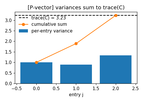
For a random vector, E{||x - E{x}||^2} equals trace(C), the sum of the per-entry variances (checked against the analytic covariance matrix C = A A^T and against np.cov).
print("[P-vector] E{||x - E x||^2} = trace(C) = sum of entry variances")
A = np.array([[1.0, 0.0, 0.0], [0.5, 0.8, 0.0], [-0.2, 0.3, 1.1]])
C = A @ A.T                                   # analytic covariance
z = rng.standard_normal((10**6, 3))
xv = z @ A.T                                  # zero-mean, covariance C
sq_dev = np.mean(np.sum((xv - xv.mean(axis=0)) ** 2, axis=1))
check("empirical E||x - Ex||^2 matches trace(C)",
      abs(sq_dev - np.trace(C)) < 2e-2)
per_entry = np.array([np.mean((xv[:, j] - xv[:, j].mean()) ** 2)
                      for j in range(3)])
check("sum of per-entry variances equals trace(C)",
      abs(per_entry.sum() - np.trace(C)) < 2e-2)
check("per-entry variances match diag(np.cov)",
      np.allclose(per_entry, np.diag(np.cov(xv.T, ddof=0)), atol=1e-9))

# ------------------------------------------------------------ preview
fig, ax = plt.subplots(1, 3, figsize=(12.5, 3.3))
ax[0].vlines(days, np.minimum(d, d.mean()), np.maximum(d, d.mean()),
             colors="gray", label="deviation")
ax[0].plot(days, np.full(d.size, d.mean()), "k--", label="sample mean 20.5")
ax[0].plot(days, d, "o", label="measurement")
ax[0].set_xlabel("day (24-30 Aug 2026)")
ax[0].set_ylabel("daily max temperature (degC)")
ax[0].set_title("[P-def] Kaisaniemi temperatures around their mean")
ax[0].legend(frameon=False)
ax[1].plot(b_train_grid, train_err)
ax[1].axvline(y_train.mean(), ls="--", c="k", label="sample mean")
ax[1].axhline(np.var(y_train), ls=":", c="C1", label="sample variance")
ax[1].set_xlabel("constant prediction b")
ax[1].set_ylabel("average of (y - b)$^2$ on the training set")
ax[1].set_title("[P-erm] ERM over constants: minimum at the sample mean")
ax[1].legend(frameon=False)
ax[2].bar(range(3), per_entry, label="per-entry variance")
ax[2].axhline(np.trace(C), ls="--", c="k",
              label=f"trace(C) = {np.trace(C):.2f}")
ax[2].plot([0, 1, 2], np.cumsum(per_entry), "o-", c="C1",
           label="cumulative sum")
ax[2].set_xlabel("entry j"); ax[2].set_ylabel("variance")
ax[2].legend(frameon=False)
ax[2].set_title("[P-vector] variances sum to trace(C)")
fig.tight_layout()
fig.savefig(OUT_DIR / "variance.png", dpi=110)
print(f"\n{sum(ok for _, ok in report)}/{len(report)} checks passed")
assert all(ok for _, ok in report)
[P-vector] E{||x - E x||^2} = trace(C) = sum of entry variances
  [ok] empirical E||x - Ex||^2 matches trace(C)
  [ok] sum of per-entry variances equals trace(C)
  [ok] per-entry variances match diag(np.cov)

17/17 checks passed
P-vector writes when the script runs