B-em writes when the script runsDictionary of Applied Machine Learning · training
Numerical companion to the entry training: it recomputes what the entry states and prints one line per check
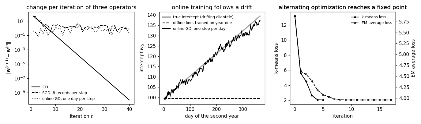
Backs the entry's view of training as an iteration w^(t+1) = T(w^(t)) whose operator T is settled by the ML setting: offline ERM by gradient descent (GD), SGD when the training set is large, online GD when data points arrive one at a time, and alternating optimization in unsupervised settings (k-means, and the EM algorithm for a GMM). Every method stops at, or near, a fixed point of its operator. Self-contained (numpy/matplotlib only), fixed seeds.
Run it without installing anything:uv run https://dictionaryofml.org/terms/training.py
uv downloads this script and the pinned NumPy and Matplotlib it needs, then runs it; the script fetches any input file it uses. To keep the output files, download training.py into a folder and run uv run training.py there. With NumPy and Matplotlib already installed, python3 training.py, from any directory — it writes its output files into the current directory. Fixed seeds, so the printed numbers reproduce exactly. Download training.py · Notebook · Open in Colab
One cell per block of the script: the code, and what that code printed when it last ran here
"""
training.py — numerical companion to the glossary entry 'training'.

Purpose
-------
Backs the entry's view of training as an iteration w^(t+1) = T(w^(t))
whose operator T is settled by the ML setting: offline ERM by gradient
descent (GD), SGD when the training set is
large, online GD when data points arrive one at a time, and alternating
optimization in unsupervised settings (k-means, and the EM algorithm for
a GMM).  Every method stops at, or near, a fixed point of its operator.
Self-contained (numpy/matplotlib only), fixed seeds.

Setup
-----
The entry's shop: daily bread demand forecast from the weather with a
linear model, demand = w1 * temperature + w0.  A year of 365 past records
is generated from a fixed line with noise; a second year with a slowly
changing clientele (the intercept drifts) supplies the online setting.
For the unsupervised settings, 300 customer profiles in the plane form
three groups.

Blocks
------
[B-gd]      Offline ERM on the year of records: T(w) = w - eta grad f(w).
            The change |w^(t+1) - w^(t)| shrinks at every iteration, and
            the iterates approach the fixed point grad f(w) = 0, the
            model parameters at which the average loss is smallest.
[B-sgd]     SGD replaces grad f by the gradient of the average loss over
            a few records; its iterates approach the same fixed point but
            the change per iteration never settles below the noise of
            the subset gradients.
[B-online]  Online GD takes one gradient step per arriving day on that
            day's loss alone; with a drifting clientele its model
            parameters follow the drift, while the offline line, fixed
            after its year, falls behind.
[B-kmeans]  Alternating optimization: assign each profile to its nearest
            cluster mean, recompute the means.  The loss never increases
            and the assignments stop changing: a fixed point.
[B-em]      The EM algorithm for a GMM alternates between the
            responsibilities of the components for each profile and the
            component parameters; the average loss (negative
            log-likelihood) never increases and the parameters settle.

Outputs
-------
training_steps.csv  : iteration, |w^(t+1) - w^(t)| for GD, SGD and online GD
training_online.csv : day of the second year, true intercept, intercept of
                      the offline line and of the online line
training_kmeans.csv : iteration, k-means loss; and training_em.csv for EM
training.png        : matplotlib preview (checking only)
"""

import numpy as np
import matplotlib

matplotlib.use("Agg")
import matplotlib.pyplot as plt

from pathlib import Path

OUT_DIR = Path(__file__).parent

report = []


def check(name, ok):
    report.append((name, bool(ok)))
    print(f"  [{'ok' if ok else 'FAIL'}] {name}")


rng = np.random.default_rng(0)
N_DAYS = 365
temp = rng.uniform(-5.0, 30.0, N_DAYS)
W_TRUE = np.array([120.0, -1.5])                 # intercept, slope: colder days, more bread
demand = W_TRUE[0] + W_TRUE[1] * temp + 6.0 * rng.standard_normal(N_DAYS)
T_MEAN, T_SD = temp.mean(), temp.std()
A = np.c_[np.ones(N_DAYS), (temp - T_MEAN) / T_SD]  # standardized temperature, for a well-conditioned f


def grad_f(w, idx=None):
    """Gradient of the average squared error loss over the records idx."""
    Ai = A if idx is None else A[idx]; yi = demand if idx is None else demand[idx]
    return 2.0 * Ai.T @ (Ai @ w - yi) / len(yi)


def loss(w):
    return float(np.mean((A @ w - demand) ** 2))
Offline ERM on the year of records: T(w) = w - eta grad f(w). The change |w^(t+1) - w^(t)| shrinks at every iteration, and the iterates approach the fixed point grad f(w) = 0, the model parameters at which the average loss is smallest.
L = 2.0 * np.linalg.eigvalsh(A.T @ A / N_DAYS).max()
ETA, T_GD = 0.5 / L, 40
w = np.zeros(2); steps_gd = []; w_gd_path = [w.copy()]
for t in range(T_GD):
    w_new = w - ETA * grad_f(w)                  # the operator T of offline ERM
    steps_gd.append(float(np.linalg.norm(w_new - w))); w = w_new; w_gd_path.append(w.copy())
w_gd = w
w_star = np.linalg.solve(A.T @ A, A.T @ demand)  # the fixed point: grad f = 0
check(f"[B-gd]      the change per iteration of GD never grows and shrinks from {steps_gd[0]:.2f} "
      f"to {steps_gd[-1]:.1e}", all(b <= a for a, b in zip(steps_gd, steps_gd[1:])) and steps_gd[-1] < 1e-6)
check(f"[B-gd]      the iterates approach the fixed point of T, where the gradient vanishes: "
      f"|grad f| = {np.linalg.norm(grad_f(w_gd)):.1e}, distance to it {np.linalg.norm(w_gd - w_star):.1e}",
      np.linalg.norm(w_gd - w_star) < 1e-3)
  [ok] [B-gd]      the change per iteration of GD never grows and shrinks from 50.34 to 9.2e-11
  [ok] [B-gd]      the iterates approach the fixed point of T, where the gradient vanishes: |grad f| = 1.8e-10, distance to it 9.2e-11
SGD replaces grad f by the gradient of the average loss over a few records; its iterates approach the same fixed point but the change per iteration never settles below the noise of the subset gradients.
BATCH = 8
w = np.zeros(2); steps_sgd = []
for t in range(T_GD):
    idx = rng.choice(N_DAYS, BATCH, replace=False)
    w_new = w - ETA * grad_f(w, idx)
    steps_sgd.append(float(np.linalg.norm(w_new - w))); w = w_new
w_sgd = w
check(f"[B-sgd]     SGD with {BATCH} records per step reaches a distance {np.linalg.norm(w_sgd - w_star):.2f} "
      f"from the fixed point (loss {loss(w_sgd):.1f} against {loss(w_star):.1f} at the fixed point)",
      loss(w_sgd) < 1.5 * loss(w_star))
check(f"[B-sgd]     its change per iteration does not settle: the last ten steps average "
      f"{np.mean(steps_sgd[-10:]):.2f}, against {np.mean(steps_gd[-10:]):.1e} for GD",
      np.mean(steps_sgd[-10:]) > 100 * np.mean(steps_gd[-10:]))
  [ok] [B-sgd]     SGD with 8 records per step reaches a distance 0.43 from the fixed point (loss 34.6 against 34.4 at the fixed point)
  [ok] [B-sgd]     its change per iteration does not settle: the last ten steps average 1.20, against 9.4e-09 for GD
Online GD takes one gradient step per arriving day on that day's loss alone; with a drifting clientele its model parameters follow the drift, while the offline line, fixed after its year, falls behind.
# a second year: the clientele changes, the true intercept drifts upward
drift = W_TRUE[0] + np.linspace(0.0, 40.0, N_DAYS)
temp2 = rng.uniform(-5.0, 30.0, N_DAYS)
demand2 = drift + W_TRUE[1] * temp2 + 6.0 * rng.standard_normal(N_DAYS)
ETA_ON = 0.05
w = w_gd.copy(); on_path = []; steps_on = []; pred_on = []; pred_off = []
for d in range(N_DAYS):
    a_d = np.array([1.0, (temp2[d] - T_MEAN) / T_SD])
    pred_on.append(float(a_d @ w)); pred_off.append(float(a_d @ w_gd))   # forecasts before the day's sales arrive
    g = 2.0 * (a_d @ w - demand2[d]) * a_d         # gradient of that day's loss alone
    w_new = w - ETA_ON * g
    steps_on.append(float(np.linalg.norm(w_new - w))); w = w_new; on_path.append(w[0])
on_path = np.array(on_path)
true_w0 = drift + W_TRUE[1] * T_MEAN              # the intercept at the mean temperature, day by day
err_offline = float(np.mean((demand2 - np.array(pred_off)) ** 2))
err_online = float(np.mean((demand2 - np.array(pred_on)) ** 2))
check(f"[B-online]  with a drifting clientele, the online line follows: its intercept ends at "
      f"{on_path[-1]:.1f} against a true {true_w0[-1]:.1f}, while the offline line stays at {w_gd[0]:.1f}",
      abs(on_path[-1] - true_w0[-1]) < abs(w_gd[0] - true_w0[-1]) / 3)
check(f"[B-online]  average loss over the second year: online {err_online:.0f}, offline {err_offline:.0f}",
      err_online < err_offline)
  [ok] [B-online]  with a drifting clientele, the online line follows: its intercept ends at 137.3 against a true 139.5, while the offline line stays at 99.5
  [ok] [B-online]  average loss over the second year: online 43, offline 554
Alternating optimization: assign each profile to its nearest cluster mean, recompute the means. The loss never increases and the assignments stop changing: a fixed point.
K = 3
centers = np.array([[0.0, 0.0], [6.0, 1.0], [3.0, 5.0]])
profiles = np.vstack([c + rng.standard_normal((100, 2)) for c in centers])
means = profiles[rng.choice(len(profiles), K, replace=False)]
km_loss = []; assign_prev = None
for t in range(50):
    d2 = ((profiles[:, None, :] - means[None]) ** 2).sum(-1)
    assign = d2.argmin(1)                         # assignment step
    km_loss.append(float(d2[np.arange(len(profiles)), assign].mean()))
    if assign_prev is not None and np.array_equal(assign, assign_prev):
        break
    means = np.array([profiles[assign == k].mean(0) for k in range(K)])  # update step
    assign_prev = assign
check(f"[B-kmeans]  the k-means loss never increases over {len(km_loss)} iterations "
      f"({km_loss[0]:.2f} -> {km_loss[-1]:.2f}) and the assignments stop changing: a fixed point",
      all(b <= a + 1e-12 for a, b in zip(km_loss, km_loss[1:])) and len(km_loss) < 50)
[ok] [B-kmeans] the k-means loss never increases over 6 iterations (13.17 -> 2.05) and the assignments stop changing: a fixed point
The EM algorithm for a GMM alternates between the responsibilities of the components for each profile and the component parameters; the average loss (negative log-likelihood) never increases and the parameters settle.
def gauss(x, mu, var):
    d = x - mu
    return np.exp(-0.5 * (d ** 2).sum(1) / var) / (2 * np.pi * var)


mu = profiles[rng.choice(len(profiles), K, replace=False)]; var = np.full(K, 2.0); pi = np.full(K, 1 / K)
em_loss = []
for t in range(100):
    dens = np.stack([pi[k] * gauss(profiles, mu[k], var[k]) for k in range(K)], 1)
    em_loss.append(float(-np.mean(np.log(dens.sum(1)))))      # average negative log-likelihood
    resp = dens / dens.sum(1, keepdims=True)                   # responsibilities of the components
    nk = resp.sum(0)
    mu_new = (resp.T @ profiles) / nk[:, None]                 # component parameters
    var_new = np.array([(resp[:, k] * ((profiles - mu_new[k]) ** 2).sum(1)).sum() / (2 * nk[k]) for k in range(K)])
    pi_new = nk / len(profiles)
    moved = float(np.abs(mu_new - mu).max()); mu, var, pi = mu_new, var_new, pi_new
    if moved < 1e-6:
        break
check(f"[B-em]      the EM algorithm's average loss never increases over {len(em_loss)} iterations "
      f"({em_loss[0]:.3f} -> {em_loss[-1]:.3f}) and the component parameters settle",
      all(b <= a + 1e-9 for a, b in zip(em_loss, em_loss[1:])) and moved < 1e-6)

# ----------------------------------------------------------------- CSV
with open(OUT_DIR / "training_steps.csv", "w") as fh:
    fh.write("iteration,gd,sgd,online\n")
    for t in range(T_GD):
        fh.write(f"{t + 1},{steps_gd[t]:.5f},{steps_sgd[t]:.5f},{steps_on[t]:.5f}\n")
with open(OUT_DIR / "training_online.csv", "w") as fh:
    fh.write("day,true_intercept,offline,online\n")
    for d in range(0, N_DAYS, 5):
        fh.write(f"{d + 1},{true_w0[d]:.3f},{w_gd[0]:.3f},{on_path[d]:.3f}\n")
with open(OUT_DIR / "training_kmeans.csv", "w") as fh:
    fh.write("iteration,loss\n")
    for t, v in enumerate(km_loss):
        fh.write(f"{t},{v:.5f}\n")
with open(OUT_DIR / "training_em.csv", "w") as fh:
    fh.write("iteration,loss\n")
    for t, v in enumerate(em_loss):
        fh.write(f"{t},{v:.5f}\n")

# -------------------------------------------------------------- preview
fig, (ax1, ax2, ax3) = plt.subplots(1, 3, figsize=(12.5, 3.7))
it = np.arange(1, T_GD + 1)
ax1.semilogy(it, steps_gd, "k-", label="GD")
ax1.semilogy(it, steps_sgd, "k--", label="SGD, 8 records per step")
ax1.semilogy(it, steps_on[:T_GD], "k:", label="online GD, one day per step")
ax1.set_xlabel("iteration $t$"); ax1.set_ylabel("$\\|\\mathbf{w}^{(t+1)} - \\mathbf{w}^{(t)}\\|$")
ax1.set_title("change per iteration of three operators"); ax1.legend(frameon=False, fontsize=8)
days = np.arange(1, N_DAYS + 1)
ax2.plot(days, true_w0, "k-", lw=2.5, alpha=0.35, label="true intercept (drifting clientele)")
ax2.plot(days, np.full(N_DAYS, w_gd[0]), "k--", label="offline line, trained on year one")
ax2.plot(days, on_path, "k-", label="online GD, one step per day")
ax2.set_xlabel("day of the second year"); ax2.set_ylabel("intercept $w_0$")
ax2.set_title("online training follows a drift"); ax2.legend(frameon=False, fontsize=8)
ax3.plot(range(len(km_loss)), km_loss, "k-o", ms=3, label="k-means loss")
ax3b = ax3.twinx(); ax3b.plot(range(len(em_loss)), em_loss, "k--s", ms=3, mfc="none", label="EM average loss")
ax3.set_xlabel("iteration"); ax3.set_ylabel("k-means loss"); ax3b.set_ylabel("EM average loss")
ax3b.set_xlabel("iteration")
ax3.set_title("alternating optimization reaches a fixed point"); ax3b.set_title(ax3.get_title())
h1, l1 = ax3.get_legend_handles_labels(); h2, l2 = ax3b.get_legend_handles_labels()
ax3.legend(h1 + h2, l1 + l2, frameon=False, fontsize=8)
fig.tight_layout()
fig.savefig(OUT_DIR / "training.png", dpi=110)

n_ok = sum(ok for _, ok in report)
print(f"\n{n_ok}/{len(report)} checks pass")
print(f"wrote {OUT_DIR / 'training_steps.csv'}, {OUT_DIR / 'training_online.csv'}, "
      f"{OUT_DIR / 'training_kmeans.csv'}, {OUT_DIR / 'training_em.csv'}, {OUT_DIR / 'training.png'}")
if n_ok != len(report):
    raise SystemExit(1)
  [ok] [B-em]      the EM algorithm's average loss never increases over 18 iterations (5.877 -> 3.955) and the component parameters settle

8/8 checks pass
wrote /Users/junga1/dictionaryappliedml/pythondemos/training_steps.csv, /Users/junga1/dictionaryappliedml/pythondemos/training_online.csv, /Users/junga1/dictionaryappliedml/pythondemos/training_kmeans.csv, /Users/junga1/dictionaryappliedml/pythondemos/training_em.csv, /Users/junga1/dictionaryappliedml/pythondemos/training.png
B-em writes when the script runs