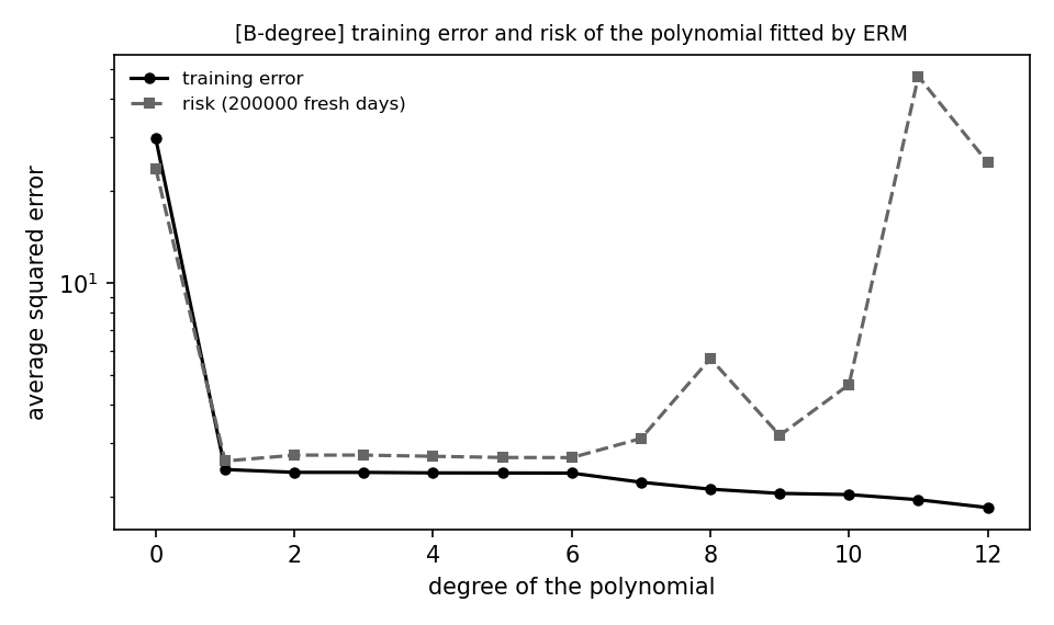
B-degree writes when the script runsDictionary of Applied Machine Learning · training error
Numerical companion to the entry training error: it recomputes what the entry states and prints one line per check
The entry's weather narrative, carried out: a straight line fitted by ERM to 40 days of synthetic weather recordings (morning minimum and maximum daytime temperature), its training error as the average of the 40 squared misses, the minimality of that average over all lines, and the training error against the risk for polynomials of growing degree fitted to the same 40 days. The days are generated exactly as in valerr.py (same seed), so the numbers of the two entries agree. Self-contained (numpy/matplotlib only), deterministic.
Run it with python3 trainerr.py, from any directory — it writes its output files into the current directory. Requires NumPy and Matplotlib only, and uses fixed seeds, so the printed numbers reproduce exactly. Download trainerr.py · Notebook · Open in Colab
One cell per block of the script: the code, and what that code printed when it last ran here
"""
trainerr.py -- numerical companion to the entry 'training error'.

The entry's weather narrative, carried out: a straight line fitted by ERM
to 40 days of synthetic weather recordings (morning minimum and maximum
daytime temperature), its training error as the average of the 40 squared
misses, the minimality of that average over all lines, and the training
error against the risk for polynomials of growing degree fitted to the same
40 days.  The days are generated exactly as in valerr.py (same seed), so the
numbers of the two entries agree.  Self-contained (numpy/matplotlib only),
deterministic.

Blocks
------
[B-def]     Fit a line to 40 days and compute its training error: the
            average squared error over the same 40 days.  Check that it is
            the average of the per-day losses and that no other line has a
            smaller one (ERM delivers the minimum).
[B-degree]  Polynomials of degree 0 to 12 fitted by ERM to the same 40
            days: the training error never increases with the degree,
            while the risk (average loss on 200000 fresh days) falls and
            then rises.  Writes the CSV behind the entry's figure.

Outputs
-------
pythondemos/trainerr_degree.csv : degree, training error and risk of the
                                  polynomial fitted by ERM.
pythondemos/trainerr.png        : preview figure (checking only).
"""

import numpy as np
import matplotlib

matplotlib.use("Agg")
import matplotlib.pyplot as plt

from pathlib import Path

OUT_DIR = Path(__file__).parent

report = []


def check(name, ok):
    report.append((name, bool(ok)))
    print(f"  [{'ok' if ok else 'FAIL'}] {name}")


def days(n, seed, noise=1.5):
    """n days: morning minimum x and maximum daytime temperature y."""
    gen = np.random.default_rng(seed)
    x = gen.uniform(-15.0, 5.0, n)
    y = 4.0 + 0.8 * x + gen.normal(0.0, noise, n)
    return x, y


def avg_sqerr(x, y, coef):
    return float(np.mean((y - np.polyval(coef, x)) ** 2))
Fit a line to 40 days and compute its training error: the average squared error over the same 40 days. Check that it is the average of the per-day losses and that no other line has a smaller one (ERM delivers the minimum).
print("[B-def] the training error of a line fitted by ERM")

x, y = days(60, seed=20260828)
tr = np.arange(40)                         # the same 40 days as in valerr.py
line = np.polyfit(x[tr], y[tr], 1)
losses = (y[tr] - np.polyval(line, x[tr])) ** 2
trainerr = avg_sqerr(x[tr], y[tr], line)
print(f"    line: slope {line[0]:.3f}, offset {line[1]:.3f}; training error "
      f"{trainerr:.3f} = average of {len(tr)} per-day squared errors "
      f"(smallest {losses.min():.3f}, largest {losses.max():.3f})")
check("the training error is the average of the per-day losses",
      np.isclose(trainerr, float(np.mean(losses)), atol=1e-12))
gen = np.random.default_rng(1)
others = line + gen.normal(0.0, [0.05, 0.5], size=(2000, 2))
worse = [avg_sqerr(x[tr], y[tr], c) for c in others]
print(f"    2000 other lines (slope and offset perturbed): smallest training "
      f"error {min(worse):.3f}")
check("no other line has a smaller training error: ERM delivers the minimum",
      min(worse) >= trainerr)
[B-def] the training error of a line fitted by ERM
    line: slope 0.903, offset 4.437; training error 2.452 = average of 40 per-day squared errors (smallest 0.000, largest 15.898)
  [ok] the training error is the average of the per-day losses
    2000 other lines (slope and offset perturbed): smallest training error 2.452
  [ok] no other line has a smaller training error: ERM delivers the minimum
Polynomials of degree 0 to 12 fitted by ERM to the same 40 days: the training error never increases with the degree, while the risk (average loss on 200000 fresh days) falls and then rises. Writes the CSV behind the entry's figure.
print("\n[B-degree] training error and risk against the degree of the polynomial")

xf, yf = days(200_000, seed=99)
DEGREES = list(range(0, 13))
rows = []
for d in DEGREES:
    coef = np.polyfit(x[tr], y[tr], d)
    rows.append((d, avg_sqerr(x[tr], y[tr], coef), avg_sqerr(xf, yf, coef)))
    print(f"    degree {d:2d}: training error {rows[-1][1]:.3f}, risk {rows[-1][2]:.3f}")
train_curve = [r[1] for r in rows]
risk_curve = [r[2] for r in rows]
check("the training error never increases with the degree",
      all(a >= b - 1e-9 for a, b in zip(train_curve, train_curve[1:])))
check("the training error is below the risk for every degree from 1 on",
      all(r[1] < r[2] for r in rows[1:]))
best = int(np.argmin(risk_curve))
print(f"    smallest risk at degree {best}; at degree 12 the training error is "
      f"{train_curve[-1]:.3f} and the risk {risk_curve[-1]:.3f}")
check("the risk is smallest at degree 1 and larger at degree 12 than at degree 1",
      best == 1 and risk_curve[-1] > risk_curve[1])

with open(OUT_DIR / "trainerr_degree.csv", "w") as fh:
    fh.write("degree,train,risk\n")
    for d, t, r in rows:
        fh.write(f"{d},{t:.4f},{r:.4f}\n")
print("    wrote trainerr_degree.csv")


# --------------------------------------------------------------- preview
fig, ax = plt.subplots(figsize=(6.4, 3.8))
ax.semilogy(DEGREES, train_curve, "o-", color="black", ms=4, label="training error")
ax.semilogy(DEGREES, risk_curve, "s--", color="0.4", ms=4, label="risk (200000 fresh days)")
ax.set_xlabel("degree of the polynomial")
ax.set_ylabel("average squared error")
ax.set_title("[B-degree] training error and risk of the polynomial fitted by ERM",
             fontsize=9)
ax.legend(frameon=False, fontsize=8)
fig.tight_layout()
fig.savefig(OUT_DIR / "trainerr.png", dpi=150)
plt.close(fig)
print("wrote trainerr.png")

passed = sum(1 for _, ok in report if ok)
print(f"\n{passed}/{len(report)} checks pass")
[B-degree] training error and risk against the degree of the polynomial
    degree  0: training error 29.665, risk 23.661
    degree  1: training error 2.452, risk 2.614
    degree  2: training error 2.401, risk 2.733
    degree  3: training error 2.400, risk 2.734
    degree  4: training error 2.391, risk 2.709
    degree  5: training error 2.389, risk 2.685
    degree  6: training error 2.387, risk 2.682
    degree  7: training error 2.228, risk 3.099
    degree  8: training error 2.115, risk 5.659
    degree  9: training error 2.049, risk 3.172
    degree 10: training error 2.030, risk 4.650
    degree 11: training error 1.953, risk 47.404
    degree 12: training error 1.841, risk 24.768
  [ok] the training error never increases with the degree
  [ok] the training error is below the risk for every degree from 1 on
    smallest risk at degree 1; at degree 12 the training error is 1.841 and the risk 24.768
  [ok] the risk is smallest at degree 1 and larger at degree 12 than at degree 1
    wrote trainerr_degree.csv
wrote trainerr.png

5/5 checks pass
B-degree writes when the script runs