B-ml writes when the script runsDictionary of Applied Machine Learning · random experiment
Numerical companion to the entry random experiment: it recomputes what the entry states and prints one line per check
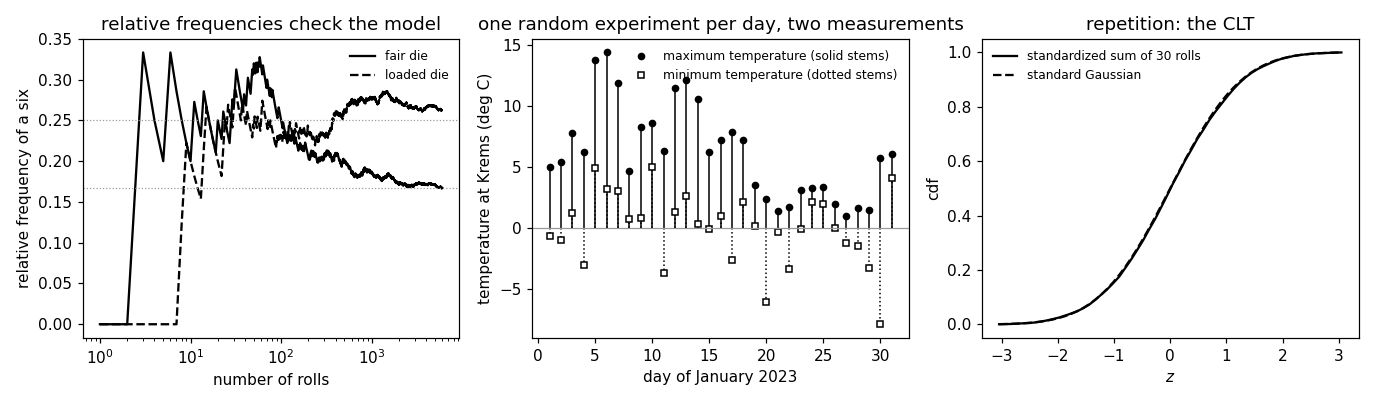
Backs the entry's claims with three random experiments: rolling a die, whose probability measure is a model that the relative frequencies of many rolls check; the weather of a day at Krems an der Donau, whose outcome is read through a random variable (RV) whose probability distribution the probability measure on the sample space induces; and the repetition of an experiment, whose outcomes are sequences, whose measurements are i.i.d. RVs, and whose long-run behavior the law of large numbers (LLN) and the central limit theorem (CLT) make precise. Self-contained (numpy/matplotlib only), fixed seed.
Run it without installing anything:uv run https://dictionaryofml.org/terms/randomexperiment.py
uv downloads this script and the pinned NumPy and Matplotlib it needs, then runs it; the script fetches any input file it uses. To keep the output files, download randomexperiment.py into a folder and run uv run randomexperiment.py there. With NumPy and Matplotlib already installed, python3 randomexperiment.py, from any directory — it writes its output files into the current directory. Fixed seeds, so the printed numbers reproduce exactly. Download randomexperiment.py · Notebook · Open in Colab
One cell per block of the script: the code, and what that code printed when it last ran here
"""
randomexperiment.py — numerical companion to the glossary entry 'random
experiment'.

Purpose
-------
Backs the entry's claims with three random experiments: rolling a die,
whose probability measure is a model that the relative frequencies of
many rolls check; the weather of a day at Krems an der Donau, whose
outcome is read through a random variable (RV) whose probability
distribution the probability measure on the sample space induces; and
the repetition of an experiment, whose outcomes are sequences, whose
measurements are i.i.d. RVs, and whose long-run behavior the law of
large numbers (LLN) and the central limit theorem (CLT) make precise.
Self-contained (numpy/matplotlib only), fixed seed.

Setup
-----
Die: sample space {1, ..., 6}; the uniform probability measure is the
model of a fair die, a second measure with P(6) = 1/4 the model of a
loaded one.  Weather: the sample space is the set of 365 days of 2023 at
Krems with the uniform measure, the RV x the maximum temperature of a
day (minimum and maximum downloaded from GeoSphere Austria); the days of
January 2023 are the entry's opening figure.  Repetition: m rolls of the
fair die, m = 1 to 5000.

Blocks
------
[B-die]     The probability measure is a property of the model, not of
            the process: 6000 rolls of a fair die and of a loaded one
            produce relative frequencies of a six near 1/6 and 1/4, and
            the frequencies tell the two models apart.
[B-january] The weather of a day at Krems as a random experiment, one
            experiment per day: the minimum and the maximum temperature of
            the 31 days of January 2023 are its measurements, the stems of
            the entry's opening figure.  Read the other way, the whole
            month is one random experiment whose outcome is the sequence.
[B-rv]      The outcome of the weather experiment is a day; the
            measurement x(omega) is its maximum temperature.  The induced
            probability distribution P^(x)(B) = P(x in B) is the fraction
            of days with x in B, checked for B = (-inf, 20].
[B-repeat]  Repeating the die m times: the outcomes are sequences, the
            product sample space has 6^m elements, the measurements are
            i.i.d. RVs.  The average of the m rolls approaches 3.5 (LLN),
            and the standardized sum of 30 rolls follows the standard
            Gaussian bell (CLT), to within 0.01 in the cdf.
[B-ml]      Two random experiments inside ML methods: the draw of a
            subset of the training set for one SGD step, whose subset
            average of the loss slopes has the full average as its
            expectation, and the bootstrap resample of a
            training set, in which a given data point appears with
            probability near 1 - 1/e.

Outputs
-------
randomexperiment_january.csv : day of January 2023 at Krems, minimum and
                            maximum temperature
randomexperiment_die.csv  : number of rolls, running relative frequency of
                            a six for the fair and the loaded die
randomexperiment_lln.csv  : m, average of m rolls
randomexperiment_clt.csv  : standardized sum of 30 rolls, its cdf over
                            10000 repetitions, and the Gaussian cdf
randomexperiment.png      : matplotlib preview (checking only)
"""

import json
import math
import urllib.request

import numpy as np
import matplotlib

matplotlib.use("Agg")
import matplotlib.pyplot as plt

from pathlib import Path

OUT_DIR = Path(__file__).parent

report = []


def check(name, ok):
    report.append((name, bool(ok)))
    print(f"  [{'ok' if ok else 'FAIL'}] {name}")


rng = np.random.default_rng(2020)
The probability measure is a property of the model, not of the process: 6000 rolls of a fair die and of a loaded one produce relative frequencies of a six near 1/6 and 1/4, and the frequencies tell the two models apart.
N_ROLLS = 6000
OMEGA = np.arange(1, 7)                              # the sample space of one roll
P_FAIR = np.full(6, 1 / 6)                           # the model of a fair die
P_LOADED = np.array([0.15, 0.15, 0.15, 0.15, 0.15, 0.25])
rolls_fair = rng.choice(OMEGA, N_ROLLS, p=P_FAIR)
rolls_loaded = rng.choice(OMEGA, N_ROLLS, p=P_LOADED)
freq_fair = np.cumsum(rolls_fair == 6) / np.arange(1, N_ROLLS + 1)
freq_loaded = np.cumsum(rolls_loaded == 6) / np.arange(1, N_ROLLS + 1)
check(f"[B-die]     after {N_ROLLS} rolls the relative frequency of a six is {freq_fair[-1]:.3f} "
      f"for the fair die (model 1/6) and {freq_loaded[-1]:.3f} for the loaded one (model 1/4)",
      abs(freq_fair[-1] - 1 / 6) < 0.02 and abs(freq_loaded[-1] - 0.25) < 0.02)
check("[B-die]     the frequencies tell the two models apart: the fair die's frequency is "
      "closer to 1/6 than to 1/4, the loaded die's the other way round",
      abs(freq_fair[-1] - 1 / 6) < abs(freq_fair[-1] - 0.25)
      and abs(freq_loaded[-1] - 0.25) < abs(freq_loaded[-1] - 1 / 6))
with open(OUT_DIR / "randomexperiment_die.csv", "w") as fh:
    fh.write("rolls,fair,loaded\n")
    for n in list(range(1, 100)) + list(range(100, N_ROLLS + 1, 20)):
        fh.write(f"{n},{freq_fair[n - 1]:.4f},{freq_loaded[n - 1]:.4f}\n")
  [ok] [B-die]     after 6000 rolls the relative frequency of a six is 0.167 for the fair die (model 1/6) and 0.262 for the loaded one (model 1/4)
  [ok] [B-die]     the frequencies tell the two models apart: the fair die's frequency is closer to 1/6 than to 1/4, the loaded die's the other way round
The weather of a day at Krems as a random experiment, one experiment per day: the minimum and the maximum temperature of the 31 days of January 2023 are its measurements, the stems of the entry's opening figure. Read the other way, the whole month is one random experiment whose outcome is the sequence.
url = ("https://dataset.api.hub.geosphere.at/v1/station/historical/"
       "klima-v2-1d?parameters=tlmin,tlmax&station_ids=3805&start=2023-01-01&end=2023-12-31")
with urllib.request.urlopen(url, timeout=120) as resp:
    rec = json.load(resp)
par = rec["features"][0]["properties"]["parameters"]
tmin = np.array(par["tlmin"]["data"], dtype=float)
tmax = np.array(par["tlmax"]["data"], dtype=float)
days = np.array(rec["timestamps"])
jan = np.array([d.startswith("2023-01") for d in days])
check(f"[B-january] {int(jan.sum())} days of January 2023 at Krems, each the outcome of one random "
      "experiment, measured by its minimum and its maximum temperature",
      jan.sum() == 31 and not np.isnan(tmin[jan]).any() and not np.isnan(tmax[jan]).any())
check(f"[B-january] the two measurements of a day are ordered, minimum below maximum, on every day "
      f"(smallest gap {np.min(tmax[jan] - tmin[jan]):.1f} degrees)", bool(np.all(tmax[jan] > tmin[jan])))
with open(OUT_DIR / "randomexperiment_january.csv", "w") as fh:
    fh.write("day,tmin,tmax\n")
    for k, (a, b) in enumerate(zip(tmin[jan], tmax[jan]), 1):
        fh.write(f"{k},{a:.1f},{b:.1f}\n")
  [ok] [B-january] 31 days of January 2023 at Krems, each the outcome of one random experiment, measured by its minimum and its maximum temperature
  [ok] [B-january] the two measurements of a day are ordered, minimum below maximum, on every day (smallest gap 1.2 degrees)
The outcome of the weather experiment is a day; the measurement x(omega) is its maximum temperature. The induced probability distribution P^(x)(B) = P(x in B) is the fraction of days with x in B, checked for B = (-inf, 20].
check(f"[B-rv]      the sample space of the weather experiment: {len(days)} days of 2023 at Krems, "
      "each an outcome omega with the uniform probability measure",
      len(days) == 365 and not np.isnan(tmax).any())
B = 20.0
induced = float(np.mean(tmax <= B))                  # P^(x)((-inf, B]) = P({omega : x(omega) <= B})
count = int((tmax <= B).sum())
check(f"[B-rv]      the RV x(omega) = maximum temperature of the day induces the distribution "
      f"P^(x)((-inf, {B:g}]) = P(x <= {B:g}) = {count}/365 = {induced:.3f}", abs(induced - count / 365) < 1e-12)
check(f"[B-rv]      the realization on 2023-07-01 is x = {tmax[181]:.1f} degrees, one value of the RV",
      days[181].startswith("2023-07-01"))
  [ok] [B-rv]      the sample space of the weather experiment: 365 days of 2023 at Krems, each an outcome omega with the uniform probability measure
  [ok] [B-rv]      the RV x(omega) = maximum temperature of the day induces the distribution P^(x)((-inf, 20]) = P(x <= 20) = 214/365 = 0.586
  [ok] [B-rv]      the realization on 2023-07-01 is x = 24.9 degrees, one value of the RV
Repeating the die m times: the outcomes are sequences, the product sample space has 6^m elements, the measurements are i.i.d. RVs. The average of the m rolls approaches 3.5 (LLN), and the standardized sum of 30 rolls follows the standard Gaussian bell (CLT), to within 0.01 in the cdf.
M_MAX = 5000
seq = rng.choice(OMEGA, M_MAX, p=P_FAIR)             # one outcome of the repeated experiment
avg = np.cumsum(seq) / np.arange(1, M_MAX + 1)
check(f"[B-repeat]  repeating the roll m times has 6^m outcomes (6^30 = {6 ** 30:.1e}); the average "
      f"of m rolls approaches 3.5: {avg[9]:.2f} at m = 10, {avg[99]:.2f} at m = 100, "
      f"{avg[-1]:.3f} at m = {M_MAX} (LLN)", abs(avg[-1] - 3.5) < 0.05)
M_CLT, REPS = 30, 10000
sums = rng.choice(OMEGA, (REPS, M_CLT), p=P_FAIR).sum(1)
mu, sd = 3.5, math.sqrt(M_CLT * 35 / 12)
# the sum takes integer values; its cdf at the integer s is compared with the
# Gaussian cdf at the standardized value of s + 1/2, the upper edge of that lattice cell
svals = np.arange(int(M_CLT * mu - 3 * sd), int(M_CLT * mu + 3 * sd) + 1)
grid = (svals + 0.5 - M_CLT * mu) / sd
emp_cdf = np.array([np.mean(sums <= sv) for sv in svals])
gauss_cdf = np.array([0.5 * (1 + math.erf(g / math.sqrt(2))) for g in grid])
gap = float(np.max(np.abs(emp_cdf - gauss_cdf)))
check(f"[B-repeat]  the standardized sum of {M_CLT} rolls follows the standard Gaussian bell: largest "
      f"gap between the cdfs over {REPS} repetitions {gap:.3f} (CLT)", gap < 0.01)
with open(OUT_DIR / "randomexperiment_lln.csv", "w") as fh:
    fh.write("m,average\n")
    for m in list(range(1, 100)) + list(range(100, M_MAX + 1, 20)):
        fh.write(f"{m},{avg[m - 1]:.4f}\n")
with open(OUT_DIR / "randomexperiment_clt.csv", "w") as fh:
    fh.write("z,cdf_sum,cdf_gauss\n")
    for g, a, b in zip(grid, emp_cdf, gauss_cdf):
        fh.write(f"{g:.3f},{a:.4f},{b:.4f}\n")
  [ok] [B-repeat]  repeating the roll m times has 6^m outcomes (6^30 = 2.2e+23); the average of m rolls approaches 3.5: 3.40 at m = 10, 3.36 at m = 100, 3.527 at m = 5000 (LLN)
  [ok] [B-repeat]  the standardized sum of 30 rolls follows the standard Gaussian bell: largest gap between the cdfs over 10000 repetitions 0.009 (CLT)
Two random experiments inside ML methods: the draw of a subset of the training set for one SGD step, whose subset average of the loss slopes has the full average as its expectation, and the bootstrap resample of a training set, in which a given data point appears with probability near 1 - 1/e.
m_train, n_sub = 365, 20
x_tr = tmax[:-1]; y_tr = tmax[1:]                    # predict tomorrow's maximum from today's
w = np.array([0.0, 0.5])
full_grad = 2 * np.mean((w[0] + w[1] * x_tr - y_tr)[:, None] * np.c_[np.ones(364), x_tr], 0)
sub_slopes = np.array([2 * np.mean((w[0] + w[1] * x_tr[i] - y_tr[i])[:, None] * np.c_[np.ones(n_sub), x_tr[i]], 0)
                       for i in (rng.choice(364, n_sub, replace=False) for _ in range(4000))])
check(f"[B-ml]      the subset draw of SGD is a random experiment with C(364, {n_sub}) outcomes; the "
      f"subset average of the loss slopes over 4000 draws, {np.round(sub_slopes.mean(0), 2)}, has the "
      f"full average {np.round(full_grad, 2)} as its expectation",
      np.allclose(sub_slopes.mean(0), full_grad, rtol=0.05, atol=0.05))
inc = np.mean([len(set(rng.integers(0, m_train, m_train))) / m_train for _ in range(2000)])
check(f"[B-ml]      a bootstrap resample of the {m_train} days holds a given day with probability "
      f"{inc:.3f}, near 1 - 1/e = {1 - 1 / math.e:.3f}", abs(inc - (1 - 1 / math.e)) < 0.01)

# -------------------------------------------------------------- preview
fig, (ax1, ax2, ax3) = plt.subplots(1, 3, figsize=(12.5, 3.7))
n = np.arange(1, N_ROLLS + 1)
ax1.plot(n, freq_fair, "k-", label="fair die"); ax1.plot(n, freq_loaded, "k--", label="loaded die")
ax1.axhline(1 / 6, color="0.6", lw=0.8, ls=":"); ax1.axhline(0.25, color="0.6", lw=0.8, ls=":")
ax1.set_xscale("log"); ax1.set_xlabel("number of rolls"); ax1.set_ylabel("relative frequency of a six")
ax1.set_title("relative frequencies check the model"); ax1.legend(frameon=False, fontsize=8)
dj = np.arange(1, 32)
ax2.vlines(dj, 0, tmax[jan], colors="k", lw=1.0)
ax2.vlines(dj, 0, tmin[jan], colors="k", lw=1.0, linestyles="dotted")
ax2.plot(dj, tmax[jan], "ko", ms=4, label="maximum temperature (solid stems)")
ax2.plot(dj, tmin[jan], "ks", ms=4, mfc="white", label="minimum temperature (dotted stems)")
ax2.axhline(0, color="0.6", lw=0.8)
ax2.set_xlabel("day of January 2023"); ax2.set_ylabel("temperature at Krems (deg C)")
ax2.set_title("one random experiment per day, two measurements"); ax2.legend(frameon=False, fontsize=8)
ax3.plot(grid, emp_cdf, "k-", label=f"standardized sum of {M_CLT} rolls")
ax3.plot(grid, gauss_cdf, "k--", label="standard Gaussian")
ax3.set_xlabel("$z$"); ax3.set_ylabel("cdf"); ax3.set_title("repetition: the CLT"); ax3.legend(frameon=False, fontsize=8)
fig.tight_layout()
fig.savefig(OUT_DIR / "randomexperiment.png", dpi=110)

n_ok = sum(ok for _, ok in report)
print(f"\n{n_ok}/{len(report)} checks pass")
print(f"wrote {OUT_DIR / 'randomexperiment_january.csv'}, {OUT_DIR / 'randomexperiment_die.csv'}, {OUT_DIR / 'randomexperiment_lln.csv'}, "
      f"{OUT_DIR / 'randomexperiment_clt.csv'}, {OUT_DIR / 'randomexperiment.png'}")
if n_ok != len(report):
    raise SystemExit(1)
  [ok] [B-ml]      the subset draw of SGD is a random experiment with C(364, 20) outcomes; the subset average of the loss slopes over 4000 draws, [ -17.49 -378.87], has the full average [ -17.47 -378.42] as its expectation
  [ok] [B-ml]      a bootstrap resample of the 365 days holds a given day with probability 0.632, near 1 - 1/e = 0.632

11/11 checks pass
wrote /Users/junga1/dictionaryappliedml/pythondemos/randomexperiment_january.csv, /Users/junga1/dictionaryappliedml/pythondemos/randomexperiment_die.csv, /Users/junga1/dictionaryappliedml/pythondemos/randomexperiment_lln.csv, /Users/junga1/dictionaryappliedml/pythondemos/randomexperiment_clt.csv, /Users/junga1/dictionaryappliedml/pythondemos/randomexperiment.png
B-ml writes when the script runs