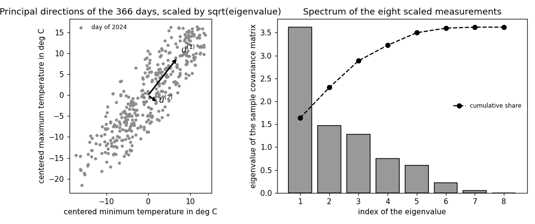
B-plot writes when the script runsDictionary of Applied Machine Learning · principal component analysis
Numerical companion to the entry principal component analysis: it recomputes what the entry states and prints one line per check
Numerical companion to the glossary entry 'pca'. The GeoSphere Austria weather station Krems (station id 3805) records eight measurements per day: minimum, maximum and mean air temperature, precipitation, sunshine duration, relative humidity, air pressure and wind speed. This script downloads the records for 2024 from the GeoSphere data hub (dataset klima-v2-1d) and writes them to pca_weather.csv. A value of -1 for precipitation marks a trace of rain too small to record and is set to 0.
Run it with python3 pca.py, from any directory — it writes its output files into the current directory. Requires NumPy and Matplotlib only, and uses fixed seeds, so the printed numbers reproduce exactly. Download pca.py · Notebook · Open in Colab
One cell per block of the script: the code, and what that code printed when it last ran here
"""Principal component analysis on a year of days at Krems: the principal
directions are the eigenvectors of the sample covariance matrix, they
maximize the variance of the projection, and the reconstruction error
they leave is the sum of the eigenvalues they drop.

Purpose
-------
Numerical companion to the glossary entry 'pca'.  The GeoSphere Austria
weather station Krems (station id 3805) records eight measurements per
day: minimum, maximum and mean air temperature, precipitation, sunshine
duration, relative humidity, air pressure and wind speed.  This script
downloads the records for 2024 from the GeoSphere data hub (dataset
klima-v2-1d) and writes them to pca_weather.csv.  A value of -1 for
precipitation marks a trace of rain too small to record and is set to 0.

Two views of the same data.  The picture uses the two temperatures in
degrees Celsius, centered but not rescaled, so the principal directions
can be drawn on the scatterplot in the units of the measurement.  The
identities use all eight measurements, each scaled to zero sample mean
and unit sample variance because temperatures, precipitation and
pressure carry different units.

The demo checks the entry's claims: (1) the first principal direction
maximizes the variance of the projection, beating two thousand random
unit vectors, and the directions are orthonormal; (2) the encoder W
built from the top eigenvectors minimizes the reconstruction error, and
that minimum equals the number of data points times the sum of the
dropped eigenvalues; (3) the decoder that minimizes the error for such
an encoder is its transpose, so the decoder is determined once the
encoder is fixed; (4) PCA is ERM with the squared error loss, its
objective value matching the average reconstruction error; and (5) the
smallest eigenvalue, four orders of magnitude below the largest, names
a redundant measurement: the mean temperature of a day is the midpoint
of its minimum and maximum.

Deterministic: the data are a fixed archive year, the decomposition is
an eigenvalue decomposition, and the random comparison vectors are
drawn with a fixed seed.  Self-contained: numpy + matplotlib only
(stdlib urllib for the download).

Blocks
------
[B-data]      Download the 366 days with eight measurements each; center
              the two temperatures for the picture and scale all eight
              for the identities.
[B-directions] Eigenvalue decomposition of the sample covariance matrix
              of the two temperatures: check the eigenvectors are
              orthonormal, that the first maximizes the variance of the
              projection against two thousand random unit vectors, and
              that the eigenvalues are those variances.
[B-reconstruct] All eight measurements, code size two: check the
              reconstruction error of the PCA encoder equals the number
              of data points times the sum of the dropped eigenvalues,
              and that no random encoder reconstructs better.
[B-decoder]   Which of the two maps may be fixed first: for a decoder
              with orthonormal columns the best encoder is its transpose,
              while a generic encoder with orthonormal rows does NOT have
              its transpose as the best decoder; and restricting the
              decoder to orthonormal columns costs nothing.
[B-trace]     The reconstruction is orthogonal to the error it leaves, so
              the reconstruction error is m times a gap between two traces;
              the second trace is maximized by the top eigenvectors.
[B-erm]       PCA as ERM: the average squared error loss of the learned
              pair equals the reconstruction error divided by the number
              of data points, and it falls as the code size grows.
[B-redundant] The smallest eigenvalue is four orders of magnitude below
              the largest, and its direction loads on the three
              temperatures alone: the mean temperature of a day is the
              midpoint of its minimum and maximum, to within the 0.05
              degree the archive records. PCA finds the redundancy
              without being told to look for one.
[B-plot]      Preview: the days in the two temperatures with the two
              principal directions, and the eigenvalue spectrum of the
              eight measurements.

Outputs
-------
pca_weather.csv    : date and the eight measurements, 366 days of 2024
pca_points.csv     : x1, x2 -- the centered temperatures of each day
pca_axis1.csv,
pca_axis2.csv      : the two principal directions as segments, scaled by
                     the square root of their eigenvalue
pca_spectrum.csv   : index, eigenvalue, cumulative share of the variance
pca.png            : preview (checking only)
"""

import json
import urllib.request
from pathlib import Path

import numpy as np
import matplotlib

matplotlib.use("Agg")
import matplotlib.pyplot as plt

OUT_DIR = Path(__file__).parent

report = []


def check(name, ok):
    report.append((name, bool(ok)))
    print(f"  [{'ok' if ok else 'FAIL'}] {name}")
Download the 366 days with eight measurements each; center the two temperatures for the picture and scale all eight for the identities.
PARAMS = ["tlmin", "tlmax", "tl_mittel", "rr", "so_h", "rf_mittel",
          "p_mittel", "vv_mittel"]
URL = ("https://dataset.api.hub.geosphere.at/v1/station/historical/"
       f"klima-v2-1d?parameters={','.join(PARAMS)}&station_ids=3805"
       "&start=2024-01-01&end=2024-12-31")
with urllib.request.urlopen(URL, timeout=120) as resp:
    payload = json.load(resp)
params = payload["features"][0]["properties"]["parameters"]
stamps = [t[:10] for t in payload["timestamps"]]
M = np.stack([np.array(params[p]["data"], dtype=float) for p in PARAMS], 1)
M[:, 3] = np.maximum(M[:, 3], 0.0)             # -1 marks a trace of rain
with open(OUT_DIR / "pca_weather.csv", "w") as f:
    f.write("date," + ",".join(PARAMS) + "\n")
    for day, row in zip(stamps, M):
        f.write(day + "," + ",".join(f"{v:g}" for v in row) + "\n")
T = M[:, :2] - M[:, :2].mean(axis=0)           # centered, in degrees
X = (M - M.mean(axis=0)) / M.std(axis=0)       # scaled, all eight
m, d = X.shape
check("[B-data] 366 days with eight measurements each", (m, d) == (366, 8))
check("[B-data] the record matches the archive (Feb 1: -3.8 to 10.4 deg)",
      stamps[31] == "2024-02-01" and np.allclose(M[31, :2], [-3.8, 10.4]))
check("[B-data] the two temperatures are centered", np.allclose(T.mean(axis=0), 0))


def principal(A):
    """Eigenvalues and eigenvectors of the sample covariance matrix of A,
    in decreasing order of eigenvalue."""
    Q = A.T @ A / len(A)
    vals, vecs = np.linalg.eigh(Q)
    order = np.argsort(vals)[::-1]
    return vals[order], vecs[:, order]
  [ok] [B-data] 366 days with eight measurements each
  [ok] [B-data] the record matches the archive (Feb 1: -3.8 to 10.4 deg)
  [ok] [B-data] the two temperatures are centered
  two temperatures: eigenvalues 130.92 and 7.94 (squared degrees); best random direction 130.92
Eigenvalue decomposition of the sample covariance matrix of the two temperatures: check the eigenvectors are orthonormal, that the first maximizes the variance of the projection against two thousand random unit vectors, and that the eigenvalues are those variances.
lam2, U2 = principal(T)
rng = np.random.default_rng(0)
angles = rng.uniform(0, 2 * np.pi, 2000)
dirs = np.stack([np.cos(angles), np.sin(angles)], 1)
var_random = ((T @ dirs.T) ** 2).mean(axis=0)
var_first = float(((T @ U2[:, 0]) ** 2).mean())
print(f"  two temperatures: eigenvalues {lam2[0]:.2f} and {lam2[1]:.2f} "
      f"(squared degrees); best random direction {var_random.max():.2f}")
check("[B-directions] the principal directions are orthonormal",
      np.allclose(U2.T @ U2, np.eye(2)))
check("[B-directions] the first maximizes the variance of the projection "
      "(2000 random unit vectors)", var_first >= var_random.max() - 1e-9)
check("[B-directions] the eigenvalues are the variances of the projections",
      np.allclose([((T @ U2[:, j]) ** 2).mean() for j in (0, 1)], lam2))
  [ok] [B-directions] the principal directions are orthonormal
  [ok] [B-directions] the first maximizes the variance of the projection (2000 random unit vectors)
  [ok] [B-directions] the eigenvalues are the variances of the projections
  eight measurements: reconstruction error 1065.6, sum of the dropped eigenvalues times m 1065.6; best of 50 random encoders 1203.3
All eight measurements, code size two: check the reconstruction error of the PCA encoder equals the number of data points times the sum of the dropped eigenvalues, and that no random encoder reconstructs better.
lam, U = principal(X)
CODE = 2
W = U[:, :CODE].T                              # encoder, CODE x d


def min_reconstruction_error(W, A):
    """min over decoders R of sum_r || a^(r) - R W a^(r) ||^2."""
    Z = A @ W.T
    R = np.linalg.lstsq(Z, A, rcond=None)[0].T
    return float(((A - Z @ R.T) ** 2).sum())


err_pca = min_reconstruction_error(W, X)
dropped = m * lam[CODE:].sum()
err_random = [min_reconstruction_error(rng.standard_normal((CODE, d)), X)
              for _ in range(50)]
print(f"  eight measurements: reconstruction error {err_pca:.1f}, sum of the "
      f"dropped eigenvalues times m {dropped:.1f}; best of 50 random "
      f"encoders {min(err_random):.1f}")
check("[B-reconstruct] the error equals m times the sum of the dropped "
      "eigenvalues", np.isclose(err_pca, dropped))
check("[B-reconstruct] no random encoder reconstructs better",
      err_pca < min(err_random))
  [ok] [B-reconstruct] the error equals m times the sum of the dropped eigenvalues
  [ok] [B-reconstruct] no random encoder reconstructs better
Which of the two maps may be fixed first: for a decoder with orthonormal columns the best encoder is its transpose, while a generic encoder with orthonormal rows does NOT have its transpose as the best decoder; and restricting the decoder to orthonormal columns costs nothing.
def best_code(R, A):
    """argmin_z || a - R z ||^2 for every row a of A, solved independently."""
    return np.linalg.lstsq(R, A.T, rcond=None)[0].T


ortho = [np.linalg.qr(rng.standard_normal((d, CODE)))[0] for _ in range(200)]
gap_dec = max(abs(float(((X - (X @ R) @ R.T) ** 2).sum())
                  - float(((X - best_code(R, X) @ R.T) ** 2).sum()))
              for R in ortho)
check("[B-decoder] for a decoder with orthonormal columns the best encoder "
      "is its transpose", gap_dec < 1e-8)

W_gen = np.linalg.qr(rng.standard_normal((d, CODE)))[0].T
Z_gen = X @ W_gen.T
R_ls = np.linalg.lstsq(Z_gen, X, rcond=None)[0].T
err_ls = float(((X - Z_gen @ R_ls.T) ** 2).sum())
err_t = float(((X - Z_gen @ W_gen) ** 2).sum())
print(f"  generic orthonormal-row encoder: its best decoder leaves "
      f"{err_ls:.1f}, its transpose {err_t:.1f}")
check("[B-decoder] a generic orthonormal-row encoder does NOT have its "
      "transpose as the best decoder", err_t > err_ls + 1.0)
Z = X @ W.T
R_hat = np.linalg.lstsq(Z, X, rcond=None)[0].T
check("[B-decoder] the eigenvector encoder does, its rows spanning an "
      "invariant subspace", np.allclose(R_hat, W.T, atol=1e-8))
free = min(min_reconstruction_error(rng.standard_normal((CODE, d)), X)
           for _ in range(300))
check("[B-decoder] no unconstrained pair beats the orthonormal-decoder "
      "optimum", free > err_pca)
  [ok] [B-decoder] for a decoder with orthonormal columns the best encoder is its transpose
  generic orthonormal-row encoder: its best decoder leaves 2003.7, its transpose 2603.4
  [ok] [B-decoder] a generic orthonormal-row encoder does NOT have its transpose as the best decoder
  [ok] [B-decoder] the eigenvector encoder does, its rows spanning an invariant subspace
  [ok] [B-decoder] no unconstrained pair beats the orthonormal-decoder optimum
The reconstruction is orthogonal to the error it leaves, so the reconstruction error is m times a gap between two traces; the second trace is maximized by the top eigenvectors.
Q = X.T @ X / m
R_top = U[:, :CODE]
pyth = float(np.abs((X ** 2).sum(1) - ((X @ R_top) ** 2).sum(1)
                    - ((X - (X @ R_top) @ R_top.T) ** 2).sum(1)).max())
check("[B-trace] the reconstruction is orthogonal to the error it leaves",
      pyth < 1e-9)
err_trace = m * (np.trace(Q) - np.trace(R_top.T @ Q @ R_top))
check("[B-trace] the reconstruction error is m times the gap between the "
      "trace of the sample covariance matrix and the projected trace",
      np.isclose(err_pca, err_trace))
best_tr = max(float(np.trace(R.T @ Q @ R)) for R in ortho)
print(f"  trace: best of {len(ortho)} random orthonormal decoders "
      f"{best_tr:.4f}, sum of the top {CODE} eigenvalues "
      f"{lam[:CODE].sum():.4f}")
check("[B-trace] no random orthonormal decoder reaches the sum of the top "
      "eigenvalues", best_tr < lam[:CODE].sum())
  [ok] [B-trace] the reconstruction is orthogonal to the error it leaves
  [ok] [B-trace] the reconstruction error is m times the gap between the trace of the sample covariance matrix and the projected trace
  trace: best of 200 random orthonormal decoders 4.0150, sum of the top 2 eigenvalues 5.0884
  [ok] [B-trace] no random orthonormal decoder reaches the sum of the top eigenvalues
PCA as ERM: the average squared error loss of the learned pair equals the reconstruction error divided by the number of data points, and it falls as the code size grows.
avg_loss = float(((X - Z @ W) ** 2).sum(axis=1).mean())
check("[B-erm] the average squared error loss equals the reconstruction "
      "error per data point", np.isclose(avg_loss, err_pca / m))
curve = [(k, m * lam[k:].sum() / m) for k in range(1, d + 1)]
check("[B-erm] the average loss falls as the code size grows",
      all(curve[i][1] > curve[i + 1][1] for i in range(len(curve) - 1)))
share = np.cumsum(lam) / lam.sum()
print("  average squared error loss by code size: "
      + ", ".join(f"{k}: {v:.2f}" for k, v in curve[:4])
      + f"; two components carry {100 * share[1]:.0f}% of the variance")
  [ok] [B-erm] the average squared error loss equals the reconstruction error per data point
  [ok] [B-erm] the average loss falls as the code size grows
  average squared error loss by code size: 1: 4.38, 2: 2.91, 3: 1.63, 4: 0.88; two components carry 64% of the variance
  smallest eigenvalue 6.47e-06 against the largest 3.62; its direction loads on tlmin, tlmax, tl_mittel; the mean temperature differs from the midpoint of minimum and maximum by at most 0.05 deg
The smallest eigenvalue is four orders of magnitude below the largest, and its direction loads on the three temperatures alone: the mean temperature of a day is the midpoint of its minimum and maximum, to within the 0.05 degree the archive records. PCA finds the redundancy without being told to look for one.
small = lam[-1]
load = U[:, -1] / np.abs(U[:, -1]).max()
named = {PARAMS[j]: float(load[j]) for j in range(d) if abs(load[j]) > 0.1}
mid = (M[:, 0] + M[:, 1]) / 2.0
gap = float(np.abs(M[:, 2] - mid).max())
print(f"  smallest eigenvalue {small:.2e} against the largest {lam[0]:.2f}; "
      f"its direction loads on {', '.join(named)}; the mean temperature "
      f"differs from the midpoint of minimum and maximum by at most "
      f"{gap:.2f} deg")
check("[B-redundant] the smallest eigenvalue is four orders of magnitude "
      "below the largest", small < 1e-4 * lam[0])
check("[B-redundant] its direction loads only on the three temperatures",
      set(named) == {"tlmin", "tlmax", "tl_mittel"})
check("[B-redundant] the mean temperature is the midpoint of the minimum and "
      "the maximum, to within the recording step",
      gap <= 0.05 + 1e-9)

# ---- CSVs for the entry's figure
np.savetxt(OUT_DIR / "pca_points.csv", T, delimiter=",", header="x1,x2",
           comments="", fmt="%.2f")
for j in (0, 1):
    tip = np.sqrt(lam2[j]) * U2[:, j] * (1.0 if U2[0, j] >= 0 else -1.0)
    with open(OUT_DIR / f"pca_axis{j + 1}.csv", "w") as f:
        f.write("x1,x2\n0.000,0.000\n" + f"{tip[0]:.3f},{tip[1]:.3f}\n")
with open(OUT_DIR / "pca_spectrum.csv", "w") as f:
    f.write("index,eigenvalue,share\n")
    for k in range(d):
        f.write(f"{k + 1},{lam[k]:.4f},{share[k]:.4f}\n")
  [ok] [B-redundant] the smallest eigenvalue is four orders of magnitude below the largest
  [ok] [B-redundant] its direction loads only on the three temperatures
  [ok] [B-redundant] the mean temperature is the midpoint of the minimum and the maximum, to within the recording step

20/20 checks pass
Preview: the days in the two temperatures with the two principal directions, and the eigenvalue spectrum of the eight measurements.
fig, (ax1, ax2) = plt.subplots(1, 2, figsize=(10, 4.2))
ax1.scatter(T[:, 0], T[:, 1], s=10, color="0.55", label="day of 2024")
for j, style in ((0, "-"), (1, "--")):
    tip = np.sqrt(lam2[j]) * U2[:, j] * (1.0 if U2[0, j] >= 0 else -1.0)
    ax1.annotate("", xy=tip, xytext=(0, 0),
                 arrowprops=dict(arrowstyle="->", lw=2, ls=style, color="black"))
    ax1.annotate(f"$u^{{({j + 1})}}$", xy=tip * 1.12, fontsize=11)
ax1.set_aspect("equal")
ax1.set_xlabel("centered minimum temperature in deg C")
ax1.set_ylabel("centered maximum temperature in deg C")
ax1.set_title("Principal directions of the 366 days, scaled by sqrt(eigenvalue)")
ax1.legend(frameon=False, fontsize=8)
ax2.bar(np.arange(1, d + 1), lam, color="0.6", edgecolor="black")
ax2.plot(np.arange(1, d + 1), share * lam.max(), "ko--", label="cumulative share")
ax2.set_xlabel("index of the eigenvalue")
ax2.set_ylabel("eigenvalue of the sample covariance matrix")
ax2.set_title("Spectrum of the eight scaled measurements")
ax2.legend(frameon=False, fontsize=8)
fig.tight_layout()
fig.savefig(OUT_DIR / "pca.png", dpi=110)

n_ok = sum(ok for _, ok in report)
print(f"\n{n_ok}/{len(report)} checks pass")
if n_ok != len(report):
    raise SystemExit(1)
B-plot writes when the script runs