B-loss writes when the script runsDictionary of Applied Machine Learning · outlier
Updated on 2026-11-19
Numerical companion to the entry outlier: it recomputes what the entry states and prints one line per check
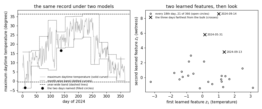
Numerical companion to the glossary entry 'outlier'. The data are the 366 days of 2024 at Krems an der Donau (GeoSphere station 3805), each day a data point with eight daily measurements. The demo recomputes the four numbers the entry states. First, a screen that calls a day unusual when its maximum daytime temperature lies more than two standard deviations from the mean gives one answer under a Gaussian model for the whole year and a different answer under a Gaussian model for the day's calendar month; the two answers disagree on most of the days either flags. Second, a bivariate Gaussian model over the morning minimum and the maximum daytime temperature ranks as the most deviating day of the year a day that neither temperature singles out on its own. Third, the eight measurements are standardized and reduced to two learned features by principal component analysis, in which the wettest day of the year sits far from every other day. Fourth, the wrong reading of one label moves a hypothesis learned by least squares much further than one learned with the absolute error loss, and the precipitation column shows that a deviating value need not be a deviating day at all: no precipitation is coded as -1 mm on 199 of the 366 days.
Run it without installing anything:uv run https://dictionaryofml.org/terms/outlier.py
uv downloads this script and the pinned NumPy and Matplotlib it needs, then runs it; the script fetches any input file it uses. To keep the output files, download outlier.py into a folder and run uv run outlier.py there. With NumPy and Matplotlib already installed, python3 outlier.py, from any directory — it writes its output files into the current directory. Fixed seeds, so the printed numbers reproduce exactly. Download outlier.py · Notebook · Open in Colab
Before running a downloaded copy, scan it: uvx bandit -q -t B102,B307,B602,B605 outlier.py (B102,B307,B602,B605 are the exec, eval and shell checks of bandit) reports nothing: the script runs no shell command and evaluates no generated code.
One cell per block of the script: the code, and what that code printed when it last ran here
"""Outliers among the daily weather records of Krems an der Donau: the same
day is an outlier under one probabilistic model and typical under another,
and two learned features make the far-out days visible.

Purpose
-------
Numerical companion to the glossary entry 'outlier'.  The data are the 366
days of 2024 at Krems an der Donau (GeoSphere station 3805), each day a
data point with eight daily measurements.  The demo recomputes the four
numbers the entry states.  First, a screen that calls a day unusual when
its maximum daytime temperature lies more than two standard deviations
from the mean gives one answer under a Gaussian model for the whole year
and a different answer under a Gaussian model for the day's calendar
month; the two answers disagree on most of the days either flags.  Second,
a bivariate Gaussian model over the morning minimum and the maximum
daytime temperature ranks as the most deviating day of the year a day that
neither temperature singles out on its own.  Third, the eight measurements
are standardized and reduced to two learned features by principal
component analysis, in which the wettest day of the year sits far from
every other day.  Fourth, the wrong reading of one label moves a
hypothesis learned by least squares much further than one learned with the
absolute error loss, and the precipitation column shows that a deviating
value need not be a deviating day at all: no precipitation is coded as
-1 mm on 199 of the 366 days.

Self-contained (numpy and matplotlib only), fixed seeds; the GeoSphere
download falls back to the committed CSV.

Blocks
------
[B-data]     The 366 days of 2024 at Krems, eight daily measurements per
             day, no missing cell.
[B-sentinel] The precipitation column codes no precipitation as -1 mm on
             199 days: what a plausibility screen flags, and what the
             code does to the annual total if it is read as an amount.
[B-model]    The maximum daytime temperature of a day under two Gaussian
             models, one for the whole year and one for its calendar
             month, with a two standard deviation screen under each.
[B-joint]    A bivariate Gaussian model over the morning minimum and the
             maximum daytime temperature: the squared Mahalanobis
             distance of each day, against the two per-feature scores.
[B-learn]    The eight standardized measurements reduced to two learned
             features by principal component analysis, and the days that
             sit apart in them.
[B-loss]     Least squares against the absolute error loss when the label
             of one day carries a transposed decimal point.

Outputs
-------
outlier_weather.csv       : date and the eight measurements (committed).
outlier_season.csv        : day of year, maximum daytime temperature, and
                            the two screen bands (year-wide, month-wise).
outlier_season_marked.csv : the two days the entry names in Fig. 1.
outlier_scores_plot.csv   : the two learned features of every 18th day,
                            21 of the 366, for the scatterplot.
outlier_scores_far.csv    : the two learned features of the three days
                            farthest from the bulk.
outlier.png               : matplotlib preview (checking only).
"""

# /// script
# requires-python = ">=3.10"
# dependencies = ["matplotlib==3.10.7", "numpy==2.3.4"]
# ///

import json
import urllib.request
from pathlib import Path

import numpy as np
import matplotlib

matplotlib.use("Agg")
import matplotlib.pyplot as plt

OUT_DIR = Path(__file__).parent

report = []


def check(name, ok):
    report.append((name, bool(ok)))
    print(f"  [{'ok' if ok else 'FAIL'}] {name}")
Installed 11 packages in 62ms
The 366 days of 2024 at Krems, eight daily measurements per day, no missing cell.
print("[B-data] the 366 days of 2024 at Krems, eight measurements per day")
NAMES = ["tlmin", "tlmax", "tl_mittel", "rr", "rf_mittel", "so_h",
         "vv_mittel", "p_mittel"]
URL = ("https://dataset.api.hub.geosphere.at/v1/station/historical/"
       "klima-v2-1d?parameters=" + ",".join(NAMES) +
       "&station_ids=3805&start=2024-01-01&end=2024-12-31")
CSV = OUT_DIR / "outlier_weather.csv"
try:
    with urllib.request.urlopen(URL, timeout=120) as resp:
        payload = json.load(resp)
    par = payload["features"][0]["properties"]["parameters"]
    dates = [stamp[:10] for stamp in payload["timestamps"]]
    raw = np.array([par[n]["data"] for n in NAMES], dtype=float).T
    with open(CSV, "w") as fh:
        fh.write("date," + ",".join(NAMES) + "\n")
        for day, row in zip(dates, raw):
            fh.write(day + "," + ",".join(f"{v:g}" for v in row) + "\n")
    print(f"    downloaded {len(dates)} days")
except OSError as err:
    print(f"    download failed ({err}); reading the committed CSV")
    lines = CSV.read_text().strip().splitlines()[1:]
    cells = [line.split(",") for line in lines]
    dates = [c[0] for c in cells]
    raw = np.array([[float(v) for v in c[1:]] for c in cells])

m = len(dates)
check(f"[B-data] {m} days, {raw.shape[1]} measurements each", m == 366)
check("[B-data] no cell is missing", bool(np.isfinite(raw).all()))
tmin = raw[:, NAMES.index("tlmin")]
tmax = raw[:, NAMES.index("tlmax")]
rain = raw[:, NAMES.index("rr")]
month = np.array([int(d[5:7]) for d in dates])
[B-data] the 366 days of 2024 at Krems, eight measurements per day
    downloaded 366 days
  [ok] [B-data] 366 days, 8 measurements each
  [ok] [B-data] no cell is missing
The precipitation column codes no precipitation as -1 mm on 199 days: what a plausibility screen flags, and what the code does to the annual total if it is read as an amount.
print("[B-sentinel] the precipitation column codes no precipitation as -1 mm")
n_sentinel = int((rain < 0).sum())
check(f"[B-sentinel] {n_sentinel} of the {m} days carry the code -1 mm, "
      f"{100 * n_sentinel / m:.0f} percent of the year; a screen that "
      f"rejects a negative amount flags every one of them",
      n_sentinel == 199)
check(f"[B-sentinel] the smallest value of the column is {rain.min():g} mm "
      f"and the largest {rain.max():g} mm", rain.min() == -1.0)
clean = np.where(rain < 0, 0.0, rain)
check(f"[B-sentinel] read as an amount, the code lowers the annual total "
      f"from {clean.sum():.1f} mm to {rain.sum():.1f} mm, by "
      f"{clean.sum() - rain.sum():.0f} mm", clean.sum() > rain.sum())
z_dry = (-1.0 - rain.mean()) / rain.std()
z_wet = (rain.max() - rain.mean()) / rain.std()
check(f"[B-sentinel] a two standard deviation screen on the column as it "
      f"stands does not flag a dry day (score {z_dry:.2f}) but does flag "
      f"the wettest day (score {z_wet:.2f})", abs(z_dry) < 2 < z_wet)
wettest = int(np.argmax(rain))
check(f"[B-sentinel] the wettest day is {dates[wettest]} with "
      f"{rain[wettest]:g} mm", dates[wettest] == "2024-09-14")
X = raw.copy()
X[:, NAMES.index("rr")] = clean
[B-sentinel] the precipitation column codes no precipitation as -1 mm
  [ok] [B-sentinel] 199 of the 366 days carry the code -1 mm, 54 percent of the year; a screen that rejects a negative amount flags every one of them
  [ok] [B-sentinel] the smallest value of the column is -1 mm and the largest 81.7 mm
  [ok] [B-sentinel] read as an amount, the code lowers the annual total from 712.0 mm to 513.0 mm, by 199 mm
  [ok] [B-sentinel] a two standard deviation screen on the column as it stands does not flag a dry day (score -0.37) but does flag the wettest day (score 12.36)
  [ok] [B-sentinel] the wettest day is 2024-09-14 with 81.7 mm
The maximum daytime temperature of a day under two Gaussian models, one for the whole year and one for its calendar month, with a two standard deviation screen under each.
print("[B-model] the same day under a year-wide and a month-wise model")
y_mean, y_sd = float(tmax.mean()), float(tmax.std())
z_year = (tmax - y_mean) / y_sd
z_month = np.zeros(m)
mon_mean = np.zeros(m)
mon_sd = np.zeros(m)
for k in range(1, 13):
    sel = month == k
    mu, sd = float(tmax[sel].mean()), float(tmax[sel].std())
    mon_mean[sel], mon_sd[sel] = mu, sd
    z_month[sel] = (tmax[sel] - mu) / sd
check(f"[B-model] year-wide model: mean {y_mean:.2f} and standard "
      f"deviation {y_sd:.2f} degrees", y_sd > 9.0)
flag_y = np.abs(z_year) > 2.0
flag_m = np.abs(z_month) > 2.0
both = flag_y & flag_m
check(f"[B-model] a two standard deviation screen flags "
      f"{int(flag_y.sum())} days under the year-wide model and "
      f"{int(flag_m.sum())} under the month-wise model, and only "
      f"{int(both.sum())} day(s) under both",
      int(both.sum()) < min(flag_y.sum(), flag_m.sum()))
j = int(np.argmin(np.where(np.abs(z_year) < 1.0, z_month, 0.0)))
check(f"[B-model] {dates[j]} has a maximum daytime temperature of "
      f"{tmax[j]:.1f} degrees: score {z_year[j]:+.2f} under the year-wide "
      f"model, {z_month[j]:+.2f} under the model for its month "
      f"(mean {mon_mean[j]:.1f}, standard deviation {mon_sd[j]:.2f}), so "
      f"only the month-wise screen flags it",
      abs(z_year[j]) < 1.0 and z_month[j] < -2.0 and flag_m[j] and
      not flag_y[j])
i = int(np.argmin(np.where(flag_y & ~flag_m, z_year, 0.0)))
check(f"[B-model] {dates[i]} runs the other way: {tmax[i]:.1f} degrees, "
      f"the coldest maximum of the year, score {z_year[i]:+.2f} under the "
      f"year-wide model and {z_month[i]:+.2f} under the model for its "
      f"month (mean {mon_mean[i]:.1f}, standard deviation "
      f"{mon_sd[i]:.2f}), so only the year-wide screen flags it",
      flag_y[i] and not flag_m[i] and tmax[i] == tmax.min())
check(f"[B-model] {int((flag_y | flag_m).sum())} days are flagged by at "
      f"least one of the two screens and only {dates[int(np.argmax(both))]} "
      f"by both", int((flag_y | flag_m).sum()) == 12)
[B-model] the same day under a year-wide and a month-wise model
  [ok] [B-model] year-wide model: mean 17.91 and standard deviation 9.20 degrees
  [ok] [B-model] a two standard deviation screen flags 3 days under the year-wide model and 10 under the month-wise model, and only 1 day(s) under both
  [ok] [B-model] 2024-05-17 has a maximum daytime temperature of 16.6 degrees: score -0.14 under the year-wide model, -2.60 under the model for its month (mean 22.3, standard deviation 2.19), so only the month-wise screen flags it
  [ok] [B-model] 2024-01-09 runs the other way: -3.6 degrees, the coldest maximum of the year, score -2.34 under the year-wide model and -1.94 under the model for its month (mean 6.0, standard deviation 4.93), so only the year-wide screen flags it
  [ok] [B-model] 12 days are flagged by at least one of the two screens and only 2024-12-31 by both
A bivariate Gaussian model over the morning minimum and the maximum daytime temperature: the squared Mahalanobis distance of each day, against the two per-feature scores.
print("[B-joint] a bivariate Gaussian model over the two temperatures")
T = np.column_stack([tmin, tmax])
t_mean = T.mean(axis=0)
t_cov = np.cov(T.T, bias=True)
corr = t_cov[0, 1] / np.sqrt(t_cov[0, 0] * t_cov[1, 1])
dev = T - t_mean
maha = np.einsum("ij,jk,ik->i", dev, np.linalg.inv(t_cov), dev)
per_feature = np.abs(dev) / np.sqrt(np.diag(t_cov))
check(f"[B-joint] the two temperatures have correlation {corr:.3f}, so the "
      f"model expects them to rise and fall together", corr > 0.8)
f = int(np.argmax(maha))
check(f"[B-joint] the largest squared Mahalanobis distance of the year, "
      f"{maha[f]:.1f}, belongs to {dates[f]}: morning minimum "
      f"{tmin[f]:.1f}, maximum {tmax[f]:.1f} degrees", maha[f] > 6.0)
check(f"[B-joint] on that day neither temperature is unusual on its own: "
      f"per-feature scores {per_feature[f, 0]:.2f} and "
      f"{per_feature[f, 1]:.2f}, both below 1",
      per_feature[f].max() < 1.0)
check(f"[B-joint] its daily range of {tmax[f] - tmin[f]:.1f} degrees is "
      f"the {int((tmax - tmin > tmax[f] - tmin[f]).sum()) + 1}-largest of "
      f"the {m} days", tmax[f] - tmin[f] > 20.0)
[B-joint] a bivariate Gaussian model over the two temperatures
  [ok] [B-joint] the two temperatures have correlation 0.880, so the model expects them to rise and fall together
  [ok] [B-joint] the largest squared Mahalanobis distance of the year, 6.7, belongs to 2024-03-29: morning minimum 0.5, maximum 21.2 degrees
  [ok] [B-joint] on that day neither temperature is unusual on its own: per-feature scores 0.91 and 0.36, both below 1
  [ok] [B-joint] its daily range of 20.7 degrees is the 4-largest of the 366 days
The eight standardized measurements reduced to two learned features by principal component analysis, and the days that sit apart in them.
print("[B-learn] the eight measurements reduced to two learned features")
Z = (X - X.mean(axis=0)) / X.std(axis=0)
cov = Z.T @ Z / m
evals, evecs = np.linalg.eigh(cov)
order = np.argsort(evals)[::-1]
evals, evecs = evals[order], evecs[:, order]
scores = Z @ evecs[:, :2]
kept = evals[:2].sum() / evals.sum()
check(f"[B-learn] the two learned features keep {100 * kept:.1f} percent "
      f"of the variance of the eight standardized measurements",
      0.6 < kept < 0.7)
check("[B-learn] the first learned feature is a temperature direction "
      f"(largest weight on {NAMES[int(np.argmax(np.abs(evecs[:, 0])))]}), "
      f"the second a wetness direction (largest weight on "
      f"{NAMES[int(np.argmax(np.abs(evecs[:, 1])))]})",
      NAMES[int(np.argmax(np.abs(evecs[:, 1])))] == "rr")
# squared distance from the bulk in the plane of the two learned features
r2 = (scores ** 2 / evals[:2]).sum(axis=1)
far = np.argsort(r2)[::-1][:3]
check(f"[B-learn] the farthest day in the two learned features is "
      f"{dates[far[0]]} at squared distance {r2[far[0]]:.1f}, against "
      f"{r2[far[1]]:.1f} for {dates[far[1]]} and {r2[far[2]]:.1f} for "
      f"{dates[far[2]]}", r2[far[0]] > 2 * r2[far[1]])
check(f"[B-learn] that day is the wettest day {dates[wettest]}, which the "
      f"screen on the precipitation column also flags",
      far[0] == wettest)
check(f"[B-learn] the remaining {m - 3} days all sit at squared distance "
      f"below {np.sort(r2)[-4]:.1f}", np.sort(r2)[-4] < r2[far[2]])
[B-learn] the eight measurements reduced to two learned features
  [ok] [B-learn] the two learned features keep 63.6 percent of the variance of the eight standardized measurements
  [ok] [B-learn] the first learned feature is a temperature direction (largest weight on tlmax), the second a wetness direction (largest weight on rr)
  [ok] [B-learn] the farthest day in the two learned features is 2024-09-14 at squared distance 50.7, against 22.9 for 2024-05-31 and 8.6 for 2024-09-13
  [ok] [B-learn] that day is the wettest day 2024-09-14, which the screen on the precipitation column also flags
  [ok] [B-learn] the remaining 363 days all sit at squared distance below 8.3
  [ok] [B-learn] the scatterplot CSV thins the year to every 18th day, 21 of the 366, and the three far days are kept separately

26/26 checks pass
Least squares against the absolute error loss when the label of one day carries a transposed decimal point.
print("[B-loss] least squares against the absolute error loss")
A = np.column_stack([np.ones(m), tmin])


def least_squares(labels):
    return np.linalg.lstsq(A, labels, rcond=None)[0]


def least_abs_dev(labels):
    """Exact minimizer of the average absolute error loss over a line.

    An optimal line through two of the data points always exists, so the
    minimum over all pairs is the minimum over all lines.
    """
    best, best_val = None, np.inf
    for a in range(m):
        for b in range(a + 1, m):
            if tmin[a] == tmin[b]:
                continue
            slope = (labels[b] - labels[a]) / (tmin[b] - tmin[a])
            inter = labels[a] - slope * tmin[a]
            val = np.abs(labels - (inter + slope * tmin)).mean()
            if val < best_val - 1e-12:
                best, best_val = (inter, slope), val
    return np.array(best)


w_ls = least_squares(tmax)
w_ad = least_abs_dev(tmax)
check(f"[B-loss] on the record as it stands, least squares learns "
      f"h(x) = {w_ls[0]:.2f} + {w_ls[1]:.3f} x and the absolute error loss "
      f"h(x) = {w_ad[0]:.2f} + {w_ad[1]:.3f} x",
      abs(w_ls[1] - w_ad[1]) < 0.1)
cold = int(np.argmin(tmin))
spoiled = tmax.copy()
spoiled[cold] = tmax[cold] * 10.0            # 3.5 degrees typed as 35
v_ls = least_squares(spoiled)
v_ad = least_abs_dev(spoiled)
move_ls = float(np.max(np.abs(A @ v_ls - A @ w_ls)))
move_ad = float(np.max(np.abs(A @ v_ad - A @ w_ad)))
check(f"[B-loss] the coldest day {dates[cold]} has morning minimum "
      f"{tmin[cold]:.1f} and maximum {tmax[cold]:.1f} degrees; recorded as "
      f"{spoiled[cold]:.1f}, it is the warmest reading of the year",
      spoiled[cold] > tmax.max())
check(f"[B-loss] that one wrong label moves the predictions of the "
      f"hypothesis learned by least squares by up to {move_ls:.2f} degrees "
      f"and leaves the one learned with the absolute error loss unchanged "
      f"(by {move_ad:.2f} degrees)", move_ls > 0.5 and move_ad < 1e-9)
huge = tmax.copy()
huge[cold] = 1000.0
u_ls = least_squares(huge)
u_ad = least_abs_dev(huge)
check(f"[B-loss] pushing the same label to 1000 degrees moves least "
      f"squares by {np.max(np.abs(A @ u_ls - A @ w_ls)):.1f} degrees, while "
      f"the hypothesis learned with the absolute error loss is still the "
      f"one learned from the correct record "
      f"({np.max(np.abs(A @ u_ad - A @ w_ad)):.2f} degrees)",
      np.max(np.abs(A @ u_ad - A @ w_ad)) < 1e-9)

# ---- CSVs for the figures
doy = np.arange(1, m + 1)
with open(OUT_DIR / "outlier_season.csv", "w") as fh:
    fh.write("doy,tmax,mlo,mhi,ylo,yhi\n")
    for t in range(m):
        fh.write(f"{doy[t]},{tmax[t]:.1f},{mon_mean[t] - 2 * mon_sd[t]:.3f},"
                 f"{mon_mean[t] + 2 * mon_sd[t]:.3f},"
                 f"{y_mean - 2 * y_sd:.3f},{y_mean + 2 * y_sd:.3f}\n")
with open(OUT_DIR / "outlier_season_marked.csv", "w") as fh:
    fh.write("doy,tmax,label\n")
    for t in (j, i):
        fh.write(f"{doy[t]},{tmax[t]:.1f},{dates[t]}\n")
thin = np.arange(0, m, 18)                   # every 18th day, 21 of the 366
with open(OUT_DIR / "outlier_scores_plot.csv", "w") as fh:
    fh.write("z1,z2,date\n")
    for t in thin:
        fh.write(f"{scores[t, 0]:.4f},{scores[t, 1]:.4f},{dates[t]}\n")
with open(OUT_DIR / "outlier_scores_far.csv", "w") as fh:
    fh.write("z1,z2,date\n")
    for t in far:
        fh.write(f"{scores[t, 0]:.4f},{scores[t, 1]:.4f},{dates[t]}\n")
check(f"[B-learn] the scatterplot CSV thins the year to every 18th day, "
      f"{len(thin)} of the {m}, and the three far days are kept separately",
      len(thin) == 21)

# ---- preview
fig, (ax1, ax2) = plt.subplots(1, 2, figsize=(9.6, 4.0))
ax1.plot(doy, tmax, color="0.6", lw=0.7, ls="-",
         label="maximum daytime temperature (solid curve)")
ax1.step(doy, mon_mean + 2 * mon_sd, where="mid", color="black", lw=1.1,
         ls=":", label="month-wise band (dotted curves)")
ax1.step(doy, mon_mean - 2 * mon_sd, where="mid", color="black", lw=1.1,
         ls=":")
ax1.axhline(y_mean + 2 * y_sd, color="black", ls="--", lw=1.0,
            label="year-wide band (dashed lines)")
ax1.axhline(y_mean - 2 * y_sd, color="black", ls="--", lw=1.0)
ax1.plot(doy[[j, i]], tmax[[j, i]], "ko", ms=6,
         label="the two days named (filled circles)")
ax1.set_xlabel("day of 2024")
ax1.set_ylabel("maximum daytime temperature (degrees)")
ax1.set_title("the same record under two models")
ax1.legend(frameon=False, fontsize=7, loc="lower center")
ax2.plot(scores[thin, 0], scores[thin, 1], "ko", ms=4, mfc="none",
         label="every 18th day, 21 of 366 (open circles)")
ax2.plot(scores[far, 0], scores[far, 1], "kx", ms=8, mew=1.6,
         label="the three days farthest from the bulk (crosses)")
for t in far:
    ax2.annotate(dates[t], (scores[t, 0], scores[t, 1]), fontsize=7,
                 textcoords="offset points", xytext=(6, -2))
ax2.set_xlabel("first learned feature $z_1$ (temperature)")
ax2.set_ylabel("second learned feature $z_2$ (wetness)")
ax2.set_title("two learned features, then look")
ax2.legend(frameon=False, fontsize=7, loc="upper left")
fig.tight_layout()
fig.savefig(OUT_DIR / "outlier.png", dpi=110)

n_ok = sum(ok for _, ok in report)
print(f"\n{n_ok}/{len(report)} checks pass")
if n_ok != len(report):
    raise SystemExit(1)
[B-loss] least squares against the absolute error loss
  [ok] [B-loss] on the record as it stands, least squares learns h(x) = 10.02 + 1.099 x and the absolute error loss h(x) = 9.84 + 1.116 x
  [ok] [B-loss] the coldest day 2024-01-21 has morning minimum -10.1 and maximum 3.5 degrees; recorded as 35.0, it is the warmest reading of the year
  [ok] [B-loss] that one wrong label moves the predictions of the hypothesis learned by least squares by up to 0.56 degrees and leaves the one learned with the absolute error loss unchanged (by 0.00 degrees)
  [ok] [B-loss] pushing the same label to 1000 degrees moves least squares by 17.7 degrees, while the hypothesis learned with the absolute error loss is still the one learned from the correct record (0.00 degrees)
B-loss writes when the script runs