B-plot writes when the script runsDictionary of Applied Machine Learning · online learning
Numerical companion to the entry online learning: it recomputes what the entry states and prints one line per check
Numerical companion to the glossary entry 'onlinelearning'. The hourly air temperature at Krems an der Donau in 2024 (GeoSphere Austria archive, station 3805) is the data stream. At hour t the data point is z^(t) = (x^(t), y^(t)): the feature vector x^(t) holds a constant one and the readings of the three previous hours, the label y^(t) is the reading of hour t. Before y^(t) is known, the current model parameters w^(t) issue the forecast <w^(t), x^(t)>; then y^(t) arrives, the squared error loss L(z^(t), w^(t)) = (y^(t) - <w^(t), x^(t)>)^2 is incurred, and the model parameters are updated. Two online methods run through the same rounds: online GD, one projected gradient step per round on the newest loss, and follow-the-leader, which after each round re-solves the least-squares problem over all data points seen so far (in closed form, by the recursive least-squares update).
Run it with python3 onlinelearning.py, from any directory — it writes its output files into the current directory. Requires NumPy and Matplotlib only, and uses fixed seeds, so the printed numbers reproduce exactly. Download onlinelearning.py · Notebook · Open in Colab
One cell per block of the script: the code, and what that code printed when it last ran here
"""Online learning on an hourly temperature stream: the round protocol,
online gradient descent against follow-the-leader with full information,
Hedge against Exp3 with bandit feedback, and the regret per round
against the best fixed choice in hindsight.

Purpose
-------
Numerical companion to the glossary entry 'onlinelearning'.  The hourly
air temperature at Krems an der Donau in 2024 (GeoSphere Austria archive,
station 3805) is the data stream.  At hour t the data point is
z^(t) = (x^(t), y^(t)): the feature vector x^(t) holds a constant one
and the readings of the three previous hours, the label y^(t) is the
reading of hour t.  Before y^(t) is known, the current model parameters
w^(t) issue the forecast <w^(t), x^(t)>; then y^(t) arrives, the squared
error loss L(z^(t), w^(t)) = (y^(t) - <w^(t), x^(t)>)^2 is incurred, and
the model parameters are updated.  Two online methods run through the
same rounds: online GD, one projected gradient step per round on the
newest loss, and follow-the-leader, which after each round re-solves
the least-squares problem over all data points seen so far (in closed
form, by the recursive least-squares update).

A second problem on the same stream has bandit feedback.  The actions
are A = 5 fixed forecasters (persistence, the reading of the previous
day, the mean of the last three readings, a linear extrapolation, and
the running mean of the year so far), the model parameters w^(t) are
the pmf over the forecasters from which one is drawn, and the loss of
round t is the absolute error of the drawn forecaster's forecast,
scaled to [0, 1].  With full information all five errors are observed
after each hour and Hedge (mirror descent on the simplex with the KL
divergence) updates the pmf; with bandit feedback only the error
of the drawn forecaster is observed, and Exp3 updates the pmf from an
importance-weighted estimate of the loss vector.

The demo checks the entry's claims: every forecast uses only data
points of earlier hours; the regret of online GD after T rounds,
relative to the model parameters that are best in hindsight, stays
below the bound D G sqrt(T) of the online GD entry, and the regret per
round falls as T grows; follow-the-leader has a smaller regret on this
stream; both forecasts beat the persistence forecast (the last reading)
on the accumulated loss; with full information, Hedge's regret against
the best single forecaster stays below sqrt(2 T log A); with bandit
feedback, Exp3's regret stays below 2 sqrt((e - 1) T A log A) and
exceeds Hedge's, the price of observing one entry of the loss vector
instead of all of them; and the regret per round of both vanishes.

Deterministic: fixed seed for Exp3's draws; the readings are fetched
from the public archive.  Self-contained: numpy + matplotlib only.

Blocks
------
[B-data]     8784 hourly readings of 2024 (station 3805), turned into
             data points with three lagged readings as features.
[B-rounds]   The round protocol for online GD: forecast, reveal, loss,
             projected gradient step onto the ball of radius D/2.
             Check that every forecast uses only earlier hours.
[B-leader]   Follow-the-leader through the same rounds by the recursive
             least-squares update; check it equals the least-squares
             solution over all data points seen so far.
[B-regret]   The regret of both methods after T rounds against the best
             fixed model parameters in hindsight, for T up to 8784, and
             the bound D G sqrt(T); check the bound, the vanishing
             regret per round, and the comparison with persistence.
[B-bandit]   Five fixed forecasters as actions; Hedge with full
             information and Exp3 with bandit feedback through the same
             rounds; regret against the best single forecaster in
             hindsight and the two bounds; check both bounds, that
             Exp3's regret exceeds Hedge's, and that both regrets per
             round vanish.
[B-figures]  Data for the entry's first two figures: three days of the
             week with an offline forecaster trained once on the first
             day and then fixed, against online GD started from zero
             at hour 0 with a constant learning rate; and
             the loss functions of five consecutive hours for a scalar
             forecaster, with the online GD iterates on them.
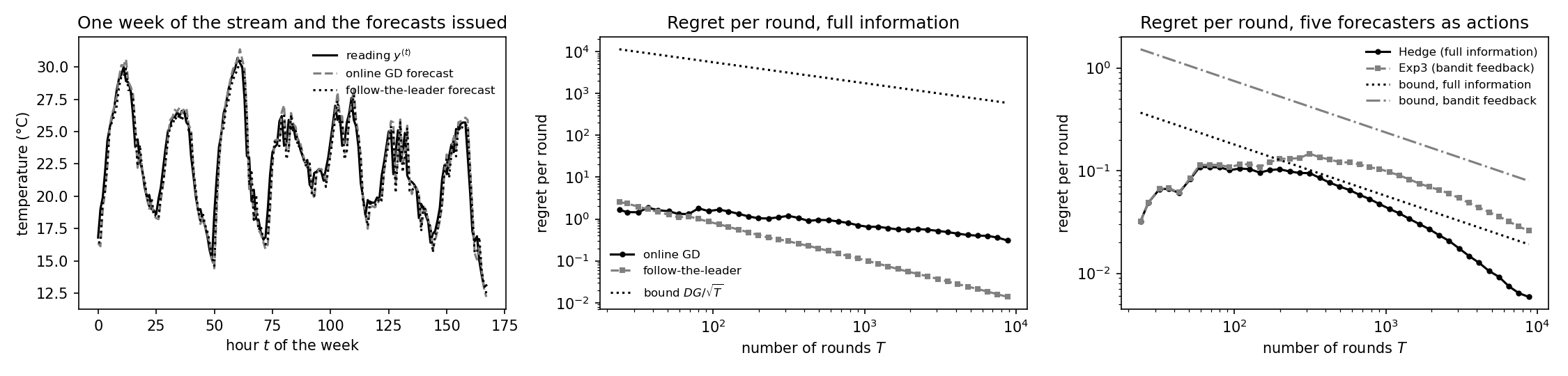
[B-plot]     Write the regret per round against T for all four methods
             and a week of forecasts, plus the preview.

Outputs
-------
onlinelearning_temperature.csv : hour, temperature -- the readings
onlinelearning_regret.csv : T, ogd, leader, bound -- regret per round
                       of online GD and follow-the-leader after T
                       rounds, and D G / sqrt(T)
onlinelearning_bandit.csv : T, hedge, exp3, hedgebound, exp3bound --
                       regret per round of Hedge (full information) and
                       Exp3 (bandit feedback) against the best single
                       forecaster, and the two bounds divided by T
onlinelearning_week.csv : hour, reading, ogd, leader -- one week of
                       readings and forecasts
onlinelearning_offline.csv : hour, reading, offline, online -- three
                       days of readings, the forecasts of a least-squares
                       forecaster trained once on the first day and then
                       fixed (nan for the first day), and the forecasts of
                       online GD started from zero at hour 0
onlinelearning_lossfuncs.csv : w, f1, ..., f5 -- the squared error loss
                       functions (y^(t) - w)^2 of five consecutive hours
                       on a grid of the scalar forecast w
onlinelearning_lossvalues.csv : t, y, w, f -- for those hours the
                       reading, the online GD iterate w^(t) and the
                       revealed value f^(t)(w^(t))
onlinelearning.png : preview (checking only)
"""

import json
import urllib.request
from pathlib import Path

import numpy as np
import matplotlib

matplotlib.use("Agg")
import matplotlib.pyplot as plt

OUT_DIR = Path(__file__).parent
ARCHIVE = "https://dataset.api.hub.geosphere.at/v1/station/historical/"
STATION = 3805

report = []                         # collects (check name, pass/fail) pairs


def check(name, ok):                # records and prints one verification
    report.append((name, bool(ok)))
    print(f"  [{'ok' if ok else 'FAIL'}] {name}")
8784 hourly readings of 2024 at station 3805; 8781 data points with a constant and 3 lagged readings as features
8784 hourly readings of 2024 (station 3805), turned into data points with three lagged readings as features.
def fetch(resource, parameter, start, end):
    """One parameter of one station from the GeoSphere Austria archive."""
    url = (f"{ARCHIVE}{resource}?parameters={parameter}"
           f"&station_ids={STATION}&start={start}&end={end}")
    with urllib.request.urlopen(url, timeout=180) as resp:
        payload = json.load(resp)
    values = payload["features"][0]["properties"]["parameters"]
    key = list(values.keys())[0]
    return (np.array(values[key]["data"], dtype=float),
            [t[:13] for t in payload["timestamps"]])


temp, stamps = fetch("klima-v2-1h", "tl", "2024-01-01T00:00", "2024-12-31T23:00")
temp = np.where(np.isnan(temp), np.nanmean(temp), temp)      # a few gaps
with open(OUT_DIR / "onlinelearning_temperature.csv", "w") as f:
    f.write("hour,temperature\n")
    for h, v in zip(stamps, temp):
        f.write(f"{h},{v:.1f}\n")
LAGS = 3
X = np.column_stack([np.ones(len(temp) - LAGS)]
                    + [temp[LAGS - k - 1:len(temp) - k - 1] for k in range(LAGS)])
y = temp[LAGS:]                                   # label: the reading of hour t
T_ALL = len(y)
print(f"  {len(temp)} hourly readings of 2024 at station {STATION}; "
      f"{T_ALL} data points with a constant and {LAGS} lagged readings as features")
check("[B-data] one data point per hour after the first three, with four features",
      X.shape == (T_ALL, LAGS + 1) and T_ALL > 8000)
  [ok] [B-data] one data point per hour after the first three, with four features
  online GD: mean squared error of the forecasts 1.71, largest gradient norm G = 928
The round protocol for online GD: forecast, reveal, loss, projected gradient step onto the ball of radius D/2. Check that every forecast uses only earlier hours.
RADIUS = 30.0                                     # W = ball of radius D/2, D = 60
D = 2.0 * RADIUS


def project(w):
    n = np.linalg.norm(w)
    return w if n <= RADIUS else w * (RADIUS / n)


def run_online_gd(X, y, lrate):
    """Forecast, reveal, loss, projected gradient step; returns the
    forecasts, the losses, the largest gradient norm and the iterates."""
    d = X.shape[1]
    w = np.zeros(d)
    forecasts, losses, G = np.empty(len(y)), np.empty(len(y)), 0.0
    for t in range(len(y)):
        forecasts[t] = w @ X[t]                   # issued before y[t] is known
        losses[t] = (y[t] - forecasts[t]) ** 2    # y[t] revealed, loss incurred
        g = -2.0 * (y[t] - forecasts[t]) * X[t]   # gradient of the newest loss
        G = max(G, float(np.linalg.norm(g)))
        w = project(w - lrate(t + 1) * g)         # the update
    return forecasts, losses, G


forecasts_ogd, losses_ogd, G = run_online_gd(X, y, lambda t: 5e-3 / np.sqrt(t))
# a second run whose stream is cut at hour 1000 must agree on the first 1000 forecasts
f_cut, _, _ = run_online_gd(X[:1000], y[:1000], lambda t: 5e-3 / np.sqrt(t))
print(f"  online GD: mean squared error of the forecasts {losses_ogd.mean():.2f}, "
      f"largest gradient norm G = {G:.0f}")
check("[B-rounds] every forecast uses only data points of earlier hours: cutting the "
      "stream at hour 1000 leaves the first 1000 forecasts unchanged",
      np.array_equal(forecasts_ogd[:1000], f_cut))
  [ok] [B-rounds] every forecast uses only data points of earlier hours: cutting the stream at hour 1000 leaves the first 1000 forecasts unchanged
  follow-the-leader: mean squared error of the forecasts 1.42; final parameters [0.242, 1.367, -0.244, -0.143] vs the minimizer over all data points [0.242, 1.367, -0.244, -0.143]
Follow-the-leader through the same rounds by the recursive least-squares update; check it equals the least-squares solution over all data points seen so far.
def run_leader(X, y, delta=1e3):
    """After each round, the least-squares minimizer over all data points
    seen so far, updated recursively (Sherman-Morrison); the forecast of
    round t uses the minimizer over rounds 1..t-1."""
    d = X.shape[1]
    w = np.zeros(d)
    P = delta * np.eye(d)                          # inverse of (X^T X + I/delta), delta large
    forecasts, losses = np.empty(len(y)), np.empty(len(y))
    for t in range(len(y)):
        forecasts[t] = w @ X[t]
        losses[t] = (y[t] - forecasts[t]) ** 2
        k = P @ X[t] / (1.0 + X[t] @ P @ X[t])
        w = w + k * (y[t] - forecasts[t])
        P = P - np.outer(k, X[t] @ P)
    return forecasts, losses, w


forecasts_ftl, losses_ftl, w_ftl = run_leader(X, y)
w_ls = np.linalg.lstsq(X, y, rcond=None)[0]
print(f"  follow-the-leader: mean squared error of the forecasts {losses_ftl.mean():.2f}; "
      f"final parameters {np.round(w_ftl, 3).tolist()} vs the minimizer over all "
      f"data points {np.round(w_ls, 3).tolist()}")
check("[B-leader] the recursive update ends at the least-squares solution over all "
      "data points (up to the tiny initial value of P)",
      np.abs(w_ftl - w_ls).max() < 1e-2)
  [ok] [B-leader] the recursive update ends at the least-squares solution over all data points (up to the tiny initial value of P)
  after T = 8781 rounds: regret of online GD 2695 (bound D G sqrt(T) = 5218846), of follow-the-leader 121; regret per round of online GD at T = 24, 168, 8784: 1.66, 1.15, 0.31; persistence forecast: mean squared error 1.81
The regret of both methods after T rounds against the best fixed model parameters in hindsight, for T up to 8784, and the bound D G sqrt(T); check the bound, the vanishing regret per round, and the comparison with persistence.
def hindsight_loss(T):
    """Accumulated loss of the best fixed w in W over the first T rounds."""
    w = np.linalg.lstsq(X[:T], y[:T], rcond=None)[0]
    assert np.linalg.norm(w) <= RADIUS            # the minimizer lies inside W
    return float(((y[:T] - X[:T] @ w) ** 2).sum())


T_GRID = np.unique(np.concatenate([np.geomspace(24, T_ALL, 40).astype(int), [T_ALL]]))
cum_ogd, cum_ftl = np.cumsum(losses_ogd), np.cumsum(losses_ftl)
regret_ogd = np.array([cum_ogd[T - 1] - hindsight_loss(T) for T in T_GRID])
regret_ftl = np.array([cum_ftl[T - 1] - hindsight_loss(T) for T in T_GRID])
bound = D * G * np.sqrt(T_GRID)
losses_persist = (y - X[:, 1]) ** 2               # forecast = the last reading
print(f"  after T = {T_ALL} rounds: regret of online GD {regret_ogd[-1]:.0f} "
      f"(bound D G sqrt(T) = {bound[-1]:.0f}), of follow-the-leader {regret_ftl[-1]:.0f}; "
      f"regret per round of online GD at T = 24, 168, 8784: "
      f"{regret_ogd[0] / T_GRID[0]:.2f}, "
      f"{regret_ogd[np.searchsorted(T_GRID, 168)] / T_GRID[np.searchsorted(T_GRID, 168)]:.2f}, "
      f"{regret_ogd[-1] / T_ALL:.2f}; persistence forecast: mean squared error "
      f"{losses_persist.mean():.2f}")
check("[B-regret] the regret of online GD stays below D G sqrt(T) for every T",
      np.all(regret_ogd <= bound))
check("[B-regret] the regret per round of online GD after all rounds is below a "
      "quarter of its value after the first day",
      regret_ogd[-1] / T_ALL < 0.25 * regret_ogd[0] / T_GRID[0])
check("[B-regret] follow-the-leader has a smaller regret than online GD after all rounds",
      regret_ftl[-1] < regret_ogd[-1])
check("[B-regret] both online methods beat the persistence forecast on the accumulated loss",
      cum_ogd[-1] < losses_persist.sum() and cum_ftl[-1] < losses_persist.sum())
  [ok] [B-regret] the regret of online GD stays below D G sqrt(T) for every T
  [ok] [B-regret] the regret per round of online GD after all rounds is below a quarter of its value after the first day
  [ok] [B-regret] follow-the-leader has a smaller regret than online GD after all rounds
  [ok] [B-regret] both online methods beat the persistence forecast on the accumulated loss
  5 forecasters; accumulated losses [820.5, 2316.2, 1387.5, 827.8, 5555.3], best single forecaster in hindsight: action 1
  after T = 8781 rounds: regret of Hedge 51.8 (bound sqrt(2 T log A) = 168.1), of Exp3 228.1 (bound 2 sqrt((e-1) T A log A) = 696.9); regret per round of Exp3 at T = 168 and 8781: 0.123, 0.026
Five fixed forecasters as actions; Hedge with full information and Exp3 with bandit feedback through the same rounds; regret against the best single forecaster in hindsight and the two bounds; check both bounds, that Exp3's regret exceeds Hedge's, and that both regrets per round vanish.
A_ACTIONS = 5
SCALE_ERR = 10.0                                  # absolute error / 10, clipped to [0, 1]
last = X[:, 1]                                    # the reading of the previous hour
day_ago = np.concatenate([last[:24], y[:-24]])    # the reading 24 hours earlier
mean3 = X[:, 1:4].mean(axis=1)                    # mean of the last three readings
extrap = 2.0 * X[:, 1] - X[:, 2]                  # linear extrapolation of the last two
running = np.concatenate([[last[0]], np.cumsum(y)[:-1] / np.arange(1, T_ALL)])
forecasters = np.column_stack([last, day_ago, mean3, extrap, running])
L = np.minimum(np.abs(y[:, None] - forecasters) / SCALE_ERR, 1.0)   # loss vectors in [0,1]^A
best_action = int(L.sum(axis=0).argmin())
print(f"  {A_ACTIONS} forecasters; accumulated losses {np.round(L.sum(axis=0), 1).tolist()}, "
      f"best single forecaster in hindsight: action {best_action + 1}")


def run_hedge(L, lrate):
    """Full information: the pmf is updated from the whole loss vector."""
    w = np.full(A_ACTIONS, 1.0 / A_ACTIONS)
    expected = np.empty(len(L))
    for t in range(len(L)):
        expected[t] = w @ L[t]                    # f^(t)(w^(t)) = <l^(t), w^(t)>
        w = w * np.exp(-lrate * L[t])
        w /= w.sum()
    return expected


def run_exp3(L, gamma, seed=0):
    """Bandit feedback: only the loss of the drawn action is observed.  The
    pmf mixes the exponential weights of the accumulated loss estimates
    with the uniform pmf (weight gamma), so every action keeps probability
    at least gamma / A and the estimates stay bounded (Auer et al. 2002)."""
    rng = np.random.default_rng(seed)
    est_total = np.zeros(A_ACTIONS)               # accumulated estimated losses
    expected = np.empty(len(L))
    for t in range(len(L)):
        weights = np.exp(-(gamma / A_ACTIONS) * (est_total - est_total.min()))
        w = (1.0 - gamma) * weights / weights.sum() + gamma / A_ACTIONS
        expected[t] = w @ L[t]                    # f^(t)(w^(t)) = <l^(t), w^(t)>
        a = rng.choice(A_ACTIONS, p=w)            # the forecaster used this hour
        est_total[a] += L[t, a] / w[a]            # unbiased estimate of l^(t)_a
    return expected


eta_hedge = np.sqrt(2.0 * np.log(A_ACTIONS) / T_ALL)
gamma_exp3 = min(1.0, np.sqrt(A_ACTIONS * np.log(A_ACTIONS) / ((np.e - 1.0) * T_ALL)))
exp_hedge, exp_exp3 = run_hedge(L, eta_hedge), run_exp3(L, gamma_exp3)
cum_hedge, cum_exp3, cum_best = np.cumsum(exp_hedge), np.cumsum(exp_exp3), np.cumsum(L, axis=0)
regret_hedge = np.array([cum_hedge[T - 1] - cum_best[T - 1].min() for T in T_GRID])
regret_exp3 = np.array([cum_exp3[T - 1] - cum_best[T - 1].min() for T in T_GRID])
bound_hedge = np.sqrt(2.0 * T_GRID * np.log(A_ACTIONS))
bound_exp3 = 2.0 * np.sqrt((np.e - 1.0) * T_GRID * A_ACTIONS * np.log(A_ACTIONS))
print(f"  after T = {T_ALL} rounds: regret of Hedge {regret_hedge[-1]:.1f} "
      f"(bound sqrt(2 T log A) = {bound_hedge[-1]:.1f}), of Exp3 {regret_exp3[-1]:.1f} "
      f"(bound 2 sqrt((e-1) T A log A) = {bound_exp3[-1]:.1f}); regret per round of "
      f"Exp3 at T = 168 and {T_ALL}: {regret_exp3[int(np.searchsorted(T_GRID, 168))] / 168:.3f}, "
      f"{regret_exp3[-1] / T_ALL:.3f}")
check("[B-bandit] with full information, Hedge's regret stays below sqrt(2 T log A) for every T",
      np.all(regret_hedge <= bound_hedge))
check("[B-bandit] with bandit feedback, Exp3's regret stays below 2 sqrt((e-1) T A log A) for every T",
      np.all(regret_exp3 <= bound_exp3))
check("[B-bandit] bandit feedback costs regret: Exp3's regret after all rounds exceeds Hedge's",
      regret_exp3[-1] > regret_hedge[-1])
i_week = int(np.searchsorted(T_GRID, 168))
check("[B-bandit] the regret per round of Hedge and Exp3 after all rounds is below half "
      "of its value after the first week",
      regret_hedge[-1] / T_ALL < 0.5 * regret_hedge[i_week] / T_GRID[i_week]
      and regret_exp3[-1] / T_ALL < 0.5 * regret_exp3[i_week] / T_GRID[i_week])
  [ok] [B-bandit] with full information, Hedge's regret stays below sqrt(2 T log A) for every T
  [ok] [B-bandit] with bandit feedback, Exp3's regret stays below 2 sqrt((e-1) T A log A) for every T
  [ok] [B-bandit] bandit feedback costs regret: Exp3's regret after all rounds exceeds Hedge's
  [ok] [B-bandit] the regret per round of Hedge and Exp3 after all rounds is below half of its value after the first week
  three days of the week: online GD from scratch has mean squared error 99 over the first six hours and 2.43 over days 2-3; the forecaster trained once on day 1 has 1.16 over days 2-3
Data for the entry's first two figures: three days of the week with an offline forecaster trained once on the first day and then fixed, against online GD started from zero at hour 0 with a constant learning rate; and the loss functions of five consecutive hours for a scalar forecaster, with the online GD iterates on them.
WEEK = slice(24 * 200, 24 * 207)                  # a week in July
DAYS3 = slice(WEEK.start, WEEK.start + 72)        # its first three days
X3, y3 = X[DAYS3], y[DAYS3]
w_offline = np.linalg.lstsq(X3[:24], y3[:24], rcond=None)[0]   # trained once on day 1
offline = X3 @ w_offline                          # then fixed for days 2 and 3
# online GD started from w = 0 at hour 0 of the window, constant learning rate:
# it forecasts from the first hour, badly at first, and adapts within the day
scratch, _, _ = run_online_gd(X3, y3, lambda t: 2e-4)
with open(OUT_DIR / "onlinelearning_offline.csv", "w") as f:
    f.write("hour,reading,offline,online\n")
    for h in range(72):
        off = f"{offline[h]:.2f}" if h >= 24 else "nan"
        f.write(f"{h},{y3[h]:.2f},{off},{scratch[h]:.2f}\n")
err_offline = np.mean((y3[24:] - offline[24:]) ** 2)
err_online = np.mean((y3[24:] - scratch[24:]) ** 2)
err_first6 = np.mean((y3[:6] - scratch[:6]) ** 2)
print(f"  three days of the week: online GD from scratch has mean squared error "
      f"{err_first6:.0f} over the first six hours and {err_online:.2f} over days 2-3; "
      f"the forecaster trained once on day 1 has {err_offline:.2f} over days 2-3")
check("[B-figures] online GD from scratch forecasts badly in the first six hours "
      "and within a factor three of the once-trained forecaster on days 2-3",
      err_first6 > 10 * err_online and err_online < 3 * err_offline)

# the scalar forecaster w of the onlineGD figure: loss (y^(t) - w)^2, update
# w^(t+1) = w^(t) - 0.2 * 2 (w^(t) - y^(t)) = 0.6 w^(t) + 0.4 y^(t)
y5 = y[WEEK][:5]
w_scalar = [y5[0]]                                # start at the first reading
for t in range(4):
    w_scalar.append(0.6 * w_scalar[-1] + 0.4 * y5[t])
w_grid = np.linspace(y5.min() - 4.0, y5.max() + 4.0, 81)
with open(OUT_DIR / "onlinelearning_lossfuncs.csv", "w") as f:
    f.write("w," + ",".join(f"f{t + 1}" for t in range(5)) + "\n")
    for wv in w_grid:
        f.write(f"{wv:.3f}," + ",".join(f"{(y5[t] - wv) ** 2:.3f}" for t in range(5)) + "\n")
with open(OUT_DIR / "onlinelearning_lossvalues.csv", "w") as f:
    f.write("t,y,w,f\n")
    for t in range(5):
        f.write(f"{t + 1},{y5[t]:.2f},{w_scalar[t]:.2f},{(y5[t] - w_scalar[t]) ** 2:.3f}\n")
check("[B-figures] each loss function of an hour is zero exactly at that hour's reading",
      all(abs((y5[t] - y5[t]) ** 2) == 0.0 and (y5[t] - w_scalar[t]) ** 2 >= 0.0 for t in range(5)))
  [ok] [B-figures] online GD from scratch forecasts badly in the first six hours and within a factor three of the once-trained forecaster on days 2-3
  [ok] [B-figures] each loss function of an hour is zero exactly at that hour's reading
Write the regret per round against T for all four methods and a week of forecasts, plus the preview.
with open(OUT_DIR / "onlinelearning_bandit.csv", "w") as f:
    f.write("T,hedge,exp3,hedgebound,exp3bound\n")
    for T, a, b, c, d in zip(T_GRID, regret_hedge, regret_exp3, bound_hedge, bound_exp3):
        f.write(f"{T},{max(a, 1e-6) / T:.6f},{max(b, 1e-6) / T:.6f},{c / T:.6f},{d / T:.6f}\n")
with open(OUT_DIR / "onlinelearning_regret.csv", "w") as f:
    f.write("T,ogd,leader,bound\n")
    for T, a, b, c in zip(T_GRID, regret_ogd, regret_ftl, bound):
        f.write(f"{T},{a / T:.4f},{b / T:.4f},{c / T:.4f}\n")
with open(OUT_DIR / "onlinelearning_week.csv", "w") as f:
    f.write("hour,reading,ogd,leader\n")
    for h, (r, a, b) in enumerate(zip(y[WEEK], forecasts_ogd[WEEK], forecasts_ftl[WEEK])):
        f.write(f"{h},{r:.2f},{a:.2f},{b:.2f}\n")

fig, axes = plt.subplots(1, 3, figsize=(15, 3.6))
ax = axes[0]
hours = np.arange(WEEK.stop - WEEK.start)
ax.plot(hours, y[WEEK], "-", color="black", label="reading $y^{(t)}$")
ax.plot(hours, forecasts_ogd[WEEK], "--", color="0.5", label="online GD forecast")
ax.plot(hours, forecasts_ftl[WEEK], ":", color="black", label="follow-the-leader forecast")
ax.set_xlabel("hour $t$ of the week")
ax.set_ylabel("temperature (°C)")
ax.set_title("One week of the stream and the forecasts issued")
ax.legend(frameon=False, fontsize=8)
ax = axes[1]
ax.plot(T_GRID, regret_ogd / T_GRID, "o-", color="black", markersize=3, label="online GD")
ax.plot(T_GRID, regret_ftl / T_GRID, "s--", color="0.5", markersize=3, label="follow-the-leader")
ax.plot(T_GRID, bound / T_GRID, ":", color="black", label="bound $DG/\\sqrt{T}$")
ax.set_xscale("log")
ax.set_yscale("log")
ax.set_xlabel("number of rounds $T$")
ax.set_ylabel("regret per round")
ax.set_title("Regret per round, full information")
ax.legend(frameon=False, fontsize=8)
ax = axes[2]
ax.plot(T_GRID, np.maximum(regret_hedge, 1e-6) / T_GRID, "o-", color="black", markersize=3,
        label="Hedge (full information)")
ax.plot(T_GRID, np.maximum(regret_exp3, 1e-6) / T_GRID, "s--", color="0.5", markersize=3,
        label="Exp3 (bandit feedback)")
ax.plot(T_GRID, bound_hedge / T_GRID, ":", color="black", label="bound, full information")
ax.plot(T_GRID, bound_exp3 / T_GRID, "-.", color="0.5", label="bound, bandit feedback")
ax.set_xscale("log")
ax.set_yscale("log")
ax.set_xlabel("number of rounds $T$")
ax.set_ylabel("regret per round")
ax.set_title("Regret per round, five forecasters as actions")
ax.legend(frameon=False, fontsize=8)
fig.tight_layout()
fig.savefig(OUT_DIR / "onlinelearning.png", dpi=150)
plt.close(fig)
check("[B-plot] the CSV files were written",
      all((OUT_DIR / f).exists() for f in
          ("onlinelearning_regret.csv", "onlinelearning_week.csv", "onlinelearning_bandit.csv",
           "onlinelearning_offline.csv", "onlinelearning_lossfuncs.csv",
           "onlinelearning_lossvalues.csv")))

passed = sum(1 for _, ok in report if ok)
print(f"\n{passed}/{len(report)} checks pass")
  [ok] [B-plot] the CSV files were written

14/14 checks pass
B-plot writes when the script runs