P-access writes when the script runsDictionary of Applied Machine Learning · loss
Numerical companion to the entry loss: it recomputes what the entry states and prints one line per check
One block per paragraph of the entry (marked [P...]): each block verifies numerically what the corresponding statement asserts. Self-contained (numpy/matplotlib only), fixed seed.
Run it without installing anything:uv run https://dictionaryofml.org/terms/loss.py
uv downloads this script and the pinned NumPy and Matplotlib it needs, then runs it; the script fetches any input file it uses. To keep the output files, download loss.py into a folder and run uv run loss.py there. With NumPy and Matplotlib already installed, python3 loss.py, from any directory — it writes its output files into the current directory. Fixed seeds, so the printed numbers reproduce exactly. Download loss.py · Notebook · Open in Colab
One cell per block of the script: the code, and what that code printed when it last ran here
"""
loss.py — numerical companion to the glossary entry 'loss'.

One block per paragraph of the entry (marked [P...]): each block verifies
numerically what the corresponding statement asserts. Self-contained
(numpy/matplotlib only), fixed seed.

Blocks
------
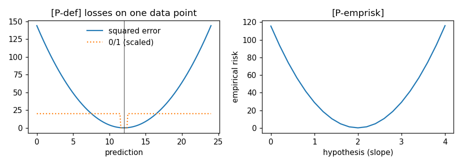
[P-def]     The loss of a hypothesis on a single data point: the entry's
            temperature example (label 12 C, prediction 8 C, squared
            error loss 16) reproduced exactly; the squared error loss
            takes a continuum of values while the 0/1 loss is binary.
[P-nonneg]  Losses built from norms are nonnegative, but nonnegativity
            is not required: the logarithmic loss -log p(y) is negative
            wherever a density exceeds one (narrow Gaussian). Losses
            exist without labels: the clustering loss (distance to the
            assigned centroid) and the autoencoder reconstruction error
            (via a rank-1 PCA reconstruction) are computed from features
            alone.
[P-emprisk] The average loss over the trainset is the empirical risk
            minimized by ERM: the least-squares fit achieves a lower
            average squared error loss than every perturbed candidate.
[P-access]  Supervised vs reinforcement learning access: with labels,
            the loss is evaluable for EVERY hypothesis on the trainset;
            in a bandit simulation only the loss of the action actually
            taken is observed, so most action-loss pairs remain
            unobserved.

Outputs
-------
loss.png : preview figure (checking only).

Data generated by pythondemos/loss.py.
"""

import numpy as np
import matplotlib

matplotlib.use("Agg")
import matplotlib.pyplot as plt
from pathlib import Path

OUT_DIR = Path(__file__).parent

rng = np.random.default_rng(42)
report = []


def check(name, ok):
    report.append((name, bool(ok)))
    print(f"  [{'ok' if ok else 'FAIL'}] {name}")
The loss of a hypothesis on a single data point: the entry's temperature example (label 12 C, prediction 8 C, squared error loss 16) reproduced exactly; the squared error loss takes a continuum of values while the 0/1 loss is binary.
print("[P-def] loss on a single data point (temperature example)")
y_true, y_pred = 12.0, 8.0
sq_loss = (y_true - y_pred) ** 2
check("squared error loss of the entry's example equals 16",
      sq_loss == 16.0)
preds = np.linspace(0, 24, 200)
sq_vals = (y_true - preds) ** 2
zo_vals = (np.round(preds) != y_true).astype(float)
check("squared error loss takes a continuum of values",
      len(np.unique(sq_vals)) > 100)
check("0/1 loss is binary", set(np.unique(zo_vals)) == {0.0, 1.0})
[P-def] loss on a single data point (temperature example)
  [ok] squared error loss of the entry's example equals 16
  [ok] squared error loss takes a continuum of values
  [ok] 0/1 loss is binary
Losses built from norms are nonnegative, but nonnegativity is not required: the logarithmic loss -log p(y) is negative wherever a density exceeds one (narrow Gaussian). Losses exist without labels: the clustering loss (distance to the assigned centroid) and the autoencoder reconstruction error (via a rank-1 PCA reconstruction) are computed from features alone.
print("[P-nonneg] nonnegativity is typical but not required")
check("norm-based loss is bounded below by zero", np.all(sq_vals >= 0))
sigma = 0.1                                        # narrow density
log_loss = -np.log(np.exp(0) / (sigma * np.sqrt(2 * np.pi)))
check("log loss is negative where the density exceeds one",
      log_loss < 0)
# unsupervised losses: clustering and autoencoder reconstruction
X = np.vstack([rng.normal(0, 0.5, (50, 2)), rng.normal(4, 0.5, (50, 2))])
centroids = np.array([[0.0, 0.0], [4.0, 4.0]])
assign = np.argmin(((X[:, None, :] - centroids) ** 2).sum(-1), axis=1)
clus_loss = np.mean(np.linalg.norm(X - centroids[assign], axis=1) ** 2)
Xc = X - X.mean(0)
u = np.linalg.svd(Xc, full_matrices=False)[2][0]   # top principal direction
recon = np.outer(Xc @ u, u)
ae_loss = np.mean(np.linalg.norm(Xc - recon, axis=1) ** 2)
check("clustering loss (distance to assigned centroid) needs no label",
      clus_loss > 0)
check("autoencoder loss = reconstruction error (rank-1 PCA)",
      ae_loss < np.mean(np.linalg.norm(Xc, axis=1) ** 2))
[P-nonneg] nonnegativity is typical but not required
  [ok] norm-based loss is bounded below by zero
  [ok] log loss is negative where the density exceeds one
  [ok] clustering loss (distance to assigned centroid) needs no label
  [ok] autoencoder loss = reconstruction error (rank-1 PCA)
The average loss over the trainset is the empirical risk minimized by ERM: the least-squares fit achieves a lower average squared error loss than every perturbed candidate.
print("[P-emprisk] average loss over the trainset = empirical risk")
mt = 80
xt = rng.uniform(0, 10, mt)
yt = 2.0 * xt + 1.0 + 0.4 * rng.normal(size=mt)
c = np.polyfit(xt, yt, 1)
risk_hat = np.mean((yt - np.polyval(c, xt)) ** 2)
check("ERM's solution minimizes the average loss (vs perturbations)",
      all(np.mean((yt - np.polyval(c + d, xt)) ** 2) > risk_hat
          for d in ([0.1, 0], [-0.1, 0], [0, 0.5], [0, -0.5])))
[P-emprisk] average loss over the trainset = empirical risk
  [ok] ERM's solution minimizes the average loss (vs perturbations)
Supervised vs reinforcement learning access: with labels, the loss is evaluable for EVERY hypothesis on the trainset; in a bandit simulation only the loss of the action actually taken is observed, so most action-loss pairs remain unobserved.
print("[P-access] loss access: supervised vs reinforcement learning")
# supervised: every hypothesis's loss is computable from the trainset
slopes = np.linspace(0, 4, 21)
sup_risks = [np.mean((yt - s * xt - 1.0) ** 2) for s in slopes]
check("supervised: the loss is evaluable for every hypothesis",
      len(sup_risks) == 21 and np.all(np.isfinite(sup_risks)))
# bandit: only the taken action's loss is revealed
true_losses = np.array([0.6, 0.4, 0.9])           # three actions
observed = np.full((300, 3), np.nan)
for t in range(300):
    a = rng.integers(3)                            # agent picks one action
    observed[t, a] = true_losses[a] + 0.1 * rng.normal()
frac_unobserved = np.isnan(observed).mean()
check("reinforcement learning: only the chosen action's loss is observed "
      "(2/3 of entries unobserved)",
      abs(frac_unobserved - 2 / 3) < 0.05)
est = np.nanmean(observed, axis=0)
check("action-loss estimates form only from observed losses",
      np.argmin(est) == np.argmin(true_losses))

# ------------------------------------------------------------ preview
fig, ax = plt.subplots(1, 2, figsize=(8.4, 3.0))
ax[0].plot(preds, sq_vals, label="squared error")
ax[0].plot(preds, 20 * zo_vals, ":", label="0/1 (scaled)")
ax[0].axvline(y_true, c="k", lw=0.5)
ax[0].set_xlabel("prediction"); ax[0].set_ylabel("loss")
ax[0].legend(frameon=False)
ax[0].set_title("[P-def] losses on one data point")
ax[1].plot(slopes, sup_risks, "-")
ax[1].set_xlabel("hypothesis (slope)"); ax[1].set_ylabel("empirical risk")
ax[1].set_title("[P-emprisk]")
fig.tight_layout()
fig.savefig(OUT_DIR / "loss.png", dpi=110)
print(f"\n{sum(ok for _, ok in report)}/{len(report)} checks passed")
assert all(ok for _, ok in report)
[P-access] loss access: supervised vs reinforcement learning
  [ok] supervised: the loss is evaluable for every hypothesis
  [ok] reinforcement learning: only the chosen action's loss is observed (2/3 of entries unobserved)
  [ok] action-loss estimates form only from observed losses

11/11 checks passed
P-access writes when the script runs