B-gd writes when the script runsDictionary of Applied Machine Learning · logistic loss
Numerical companion to the entry logistic loss: it recomputes what the entry states and prints one line per check
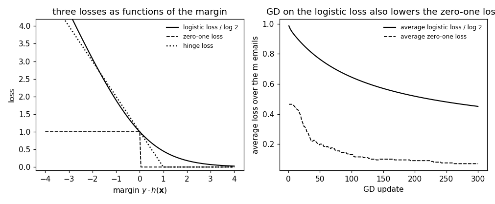
Backs the entry's claims about the logistic loss numerically: divided by log 2 it is an upper bound on the zero-one loss with equality at margin 0; it is convex and differentiable everywhere while the hinge loss has a kink at margin 1; the average zero-one loss is flat almost everywhere in the model parameters, so GD gets no direction from it, whereas GD on the average logistic loss decreases it at every step and thereby also drives the zero-one loss down. Self-contained (numpy and matplotlib only), fixed seed.
Run it without installing anything:uv run https://dictionaryofml.org/terms/logloss.py
uv downloads this script and the pinned NumPy and Matplotlib it needs, then runs it; the script fetches any input file it uses. To keep the output files, download logloss.py into a folder and run uv run logloss.py there. With NumPy and Matplotlib already installed, python3 logloss.py, from any directory — it writes its output files into the current directory. Fixed seeds, so the printed numbers reproduce exactly. Download logloss.py · Notebook · Open in Colab
One cell per block of the script: the code, and what that code printed when it last ran here
"""
logloss.py — numerical companion to the glossary entry 'logistic loss'.

Purpose
-------
Backs the entry's claims about the logistic loss numerically: divided by
log 2 it is an upper bound on the zero-one loss with equality at margin 0;
it is convex and differentiable everywhere while the hinge loss has a kink
at margin 1; the average zero-one loss is flat almost everywhere in the
model parameters, so GD gets no direction from it, whereas GD on the
average logistic loss decreases it at every step and thereby also drives
the zero-one loss down.  Self-contained (numpy and matplotlib only), fixed
seed.

Setup
-----
A spam filter as binary classification: m = 200 emails, each with two
features (a count of suspicious words and a count of links, scaled to
[0, 1]) and a label y in {-1, +1}.  The linear hypothesis h(x) = w^T x + b
is trained by ERM with the logistic loss, using GD with 300 updates that
subtract 0.5 times the gradient of the average logistic loss.

Blocks
------
[B-bound] On a grid of margins, log(1 + exp(-margin)) / log 2 is at least
          the zero-one loss everywhere, equal to it at margin 0 and
          strictly above it elsewhere.
[B-kink]  The hinge loss has different one-sided slopes at margin 1 (-1 and
          0); the logistic loss has the same one-sided slopes at every
          margin (differentiable everywhere).
[B-flat]  Starting from random model parameters, 200 small random changes
          of the parameters leave the average zero-one loss unchanged in
          at least 95 percent of the cases and the average logistic loss
          unchanged in none: the zero-one loss is flat almost everywhere
          and gives GD no direction.
[B-gd]    GD on the average logistic loss decreases it at every one of the
          300 updates; at the end the average zero-one loss is below 0.1
          and lies below the rescaled logistic loss, as the bound promises.

Outputs
-------
logloss_margin.csv : margin, logistic loss divided by log 2, zero-one loss
                     and hinge loss on a grid of margins.
logloss_gd.csv     : update index, average logistic loss divided by log 2
                     and average zero-one loss along the GD run.
logloss.png        : matplotlib preview of both panels (checking only).
"""

import numpy as np
import matplotlib

matplotlib.use("Agg")
import matplotlib.pyplot as plt

from pathlib import Path

OUT_DIR = Path(__file__).parent

report = []


def check(name, ok):
    report.append((name, bool(ok)))
    print(f"  [{'ok' if ok else 'FAIL'}] {name}")


rng = np.random.default_rng(0)
LOG2 = np.log(2.0)


def logistic(margin):
    return np.log1p(np.exp(-margin))


def zero_one(margin):
    return (margin <= 0).astype(float)


def hinge(margin):
    return np.maximum(0.0, 1.0 - margin)
On a grid of margins, log(1 + exp(-margin)) / log 2 is at least the zero-one loss everywhere, equal to it at margin 0 and strictly above it elsewhere.
mg = np.linspace(-4.0, 4.0, 161)
rescaled = logistic(mg) / LOG2
gap = rescaled - zero_one(mg)
at_zero = abs(logistic(0.0) / LOG2 - 1.0)
check(f"[B-bound] logistic loss / log 2 >= zero-one loss on the grid "
      f"(smallest gap {gap.min():.2e}), equality at margin 0 "
      f"(|difference| {at_zero:.1e})",
      gap.min() >= -1e-12 and at_zero < 1e-12
      and (gap[np.abs(mg) > 1e-9] > 0).all())
[ok] [B-bound] logistic loss / log 2 >= zero-one loss on the grid (smallest gap 0.00e+00), equality at margin 0 (|difference| 0.0e+00)
The hinge loss has different one-sided slopes at margin 1 (-1 and 0); the logistic loss has the same one-sided slopes at every margin (differentiable everywhere).
eps = 1e-6
hinge_left = (hinge(1.0) - hinge(1.0 - eps)) / eps
hinge_right = (hinge(1.0 + eps) - hinge(1.0)) / eps
log_slopes = [((logistic(t) - logistic(t - eps)) / eps,
               (logistic(t + eps) - logistic(t)) / eps)
              for t in (-2.0, 0.0, 1.0, 2.0)]
max_jump = max(abs(a - b) for a, b in log_slopes)
check(f"[B-kink]  hinge loss slopes at margin 1: {hinge_left:+.2f} (left) "
      f"vs {hinge_right:+.2f} (right); logistic loss: largest one-sided "
      f"slope difference {max_jump:.1e}",
      abs(hinge_left + 1.0) < 1e-4 and abs(hinge_right) < 1e-4
      and max_jump < 1e-4)
[ok] [B-kink] hinge loss slopes at margin 1: -1.00 (left) vs +0.00 (right); logistic loss: largest one-sided slope difference 2.5e-07
Starting from random model parameters, 200 small random changes of the parameters leave the average zero-one loss unchanged in at least 95 percent of the cases and the average logistic loss unchanged in none: the zero-one loss is flat almost everywhere and gives GD no direction.
m = 200
X = rng.uniform(0.0, 1.0, (m, 2))
y = np.where(0.8 * X[:, 0] + 1.1 * X[:, 1] - 0.9
             + 0.08 * rng.standard_normal(m) > 0, 1.0, -1.0)
Xb = np.c_[X, np.ones(m)]                      # (x1, x2, 1): w and b in one


def avg_zero_one(w):
    return float(np.mean(zero_one(y * (Xb @ w))))


def avg_logistic(w):
    return float(np.mean(logistic(y * (Xb @ w))))


w_rand = rng.standard_normal(3)
same_zo = sum(avg_zero_one(w_rand + 1e-4 * rng.standard_normal(3))
              == avg_zero_one(w_rand) for _ in range(200))
same_lg = sum(avg_logistic(w_rand + 1e-4 * rng.standard_normal(3))
              == avg_logistic(w_rand) for _ in range(200))
check(f"[B-flat]  small random changes of the model parameters leave the "
      f"average zero-one loss unchanged in {same_zo}/200 cases, the "
      f"average logistic loss in {same_lg}/200",
      same_zo >= 190 and same_lg == 0)
[ok] [B-flat] small random changes of the model parameters leave the average zero-one loss unchanged in 200/200 cases, the average logistic loss in 0/200
GD on the average logistic loss decreases it at every one of the 300 updates; at the end the average zero-one loss is below 0.1 and lies below the rescaled logistic loss, as the bound promises.
w = np.zeros(3)
n_updates = 300
trace_lg, trace_zo = [], []
for t in range(n_updates):
    margin = y * (Xb @ w)
    grad = -(Xb * (y / (1.0 + np.exp(margin)))[:, None]).mean(axis=0)
    w = w - 0.5 * grad
    trace_lg.append(avg_logistic(w) / LOG2)
    trace_zo.append(avg_zero_one(w))
decreasing = all(b < a for a, b in zip(trace_lg[:-1], trace_lg[1:]))
check(f"[B-gd]    GD lowers the average logistic loss at every update "
      f"({trace_lg[0]:.3f} -> {trace_lg[-1]:.3f}); final average zero-one "
      f"loss {trace_zo[-1]:.3f} <= rescaled logistic loss {trace_lg[-1]:.3f}",
      decreasing and trace_zo[-1] < 0.1 and trace_zo[-1] <= trace_lg[-1])

# ---------------------------------------------------------------- CSV
with open(OUT_DIR / "logloss_margin.csv", "w") as fh:
    fh.write("margin,logistic_rescaled,zeroone,hinge\n")
    for a, b, c, d in zip(mg, rescaled, zero_one(mg), hinge(mg)):
        fh.write(f"{a:.3f},{b:.4f},{c:.1f},{d:.4f}\n")
with open(OUT_DIR / "logloss_gd.csv", "w") as fh:
    fh.write("update,logistic_rescaled,zeroone\n")
    for t, (a, b) in enumerate(zip(trace_lg, trace_zo), start=1):
        fh.write(f"{t},{a:.4f},{b:.4f}\n")

# -------------------------------------------------------------- preview
fig, (ax1, ax2) = plt.subplots(1, 2, figsize=(9.2, 3.8))
ax1.plot(mg, rescaled, "k-", lw=1.4, label="logistic loss / log 2")
ax1.plot(mg, zero_one(mg), "k--", lw=1.2, label="zero-one loss")
ax1.plot(mg, hinge(mg), "k:", lw=1.6, label="hinge loss")
ax1.set_xlabel("margin $y \\cdot h(\\mathbf{x})$")
ax1.set_ylabel("loss")
ax1.set_ylim(-0.1, 4.2)
ax1.set_title("three losses as functions of the margin")
ax1.legend(frameon=False, fontsize=8)
ax2.plot(range(1, n_updates + 1), trace_lg, "k-", lw=1.4,
         label="average logistic loss / log 2")
ax2.plot(range(1, n_updates + 1), trace_zo, "k--", lw=1.2,
         label="average zero-one loss")
ax2.set_xlabel("GD update")
ax2.set_ylabel("average loss over the m emails")
ax2.set_title("GD on the logistic loss also lowers the zero-one loss")
ax2.legend(frameon=False, fontsize=8)
fig.tight_layout()
fig.savefig(OUT_DIR / "logloss.png", dpi=110)

n_ok = sum(ok for _, ok in report)
print(f"\n{n_ok}/{len(report)} checks pass")
print(f"wrote {OUT_DIR / 'logloss_margin.csv'}, {OUT_DIR / 'logloss_gd.csv'}, "
      f"{OUT_DIR / 'logloss.png'}")
if n_ok != len(report):
    raise SystemExit(1)
  [ok] [B-gd]    GD lowers the average logistic loss at every update (0.986 -> 0.451); final average zero-one loss 0.070 <= rescaled logistic loss 0.451

4/4 checks pass
wrote /Users/junga1/dictionaryappliedml/pythondemos/logloss_margin.csv, /Users/junga1/dictionaryappliedml/pythondemos/logloss_gd.csv, /Users/junga1/dictionaryappliedml/pythondemos/logloss.png
B-gd writes when the script runs