P-reg writes when the script runsDictionary of Applied Machine Learning · Gaussian random variable (Gaussian RV)
Numerical companion to the entry Gaussian random variable (Gaussian RV): it recomputes what the entry states and prints one line per check
One block per paragraph of the entry (marked [P...]), in entry order: each block verifies numerically what the corresponding paragraph asserts. Self-contained (numpy/matplotlib only, math.erf for the CDF), fixed seed.
Run it without installing anything:uv run https://dictionaryofml.org/terms/gaussrv.py
uv downloads this script and the pinned NumPy and Matplotlib it needs, then runs it; the script fetches any input file it uses. To keep the output files, download gaussrv.py into a folder and run uv run gaussrv.py there. With NumPy and Matplotlib already installed, python3 gaussrv.py, from any directory — it writes its output files into the current directory. Fixed seeds, so the printed numbers reproduce exactly. Download gaussrv.py · Notebook · Open in Colab
One cell per block of the script: the code, and what that code printed when it last ran here
"""
gaussrv.py — numerical companion to the glossary entry 'gaussrv'.

One block per paragraph of the entry (marked [P...]), in entry order: each
block verifies numerically what the corresponding paragraph asserts.
Self-contained (numpy/matplotlib only, math.erf for the CDF), fixed seed.

Blocks
------
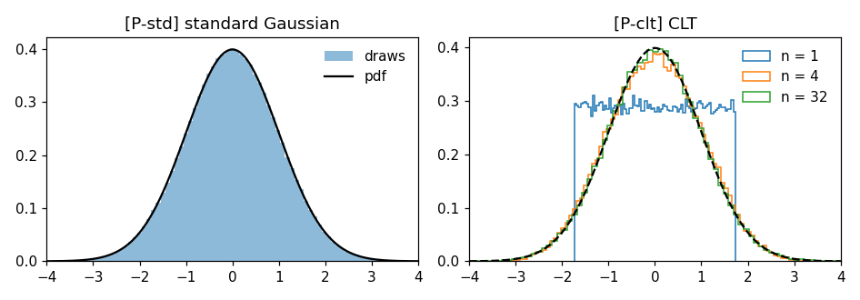
[P-def]   A standard Gaussian RV z has the pdf p(eta) = exp(-eta^2/2)/
          sqrt(2 pi): it integrates to 1 and peaks at 1/sqrt(2 pi). The
          general Gaussian RV x := sigma z + mu has mean mu and variance
          sigma^2, and the fraction of its realizations below eta matches
          Phi((eta - mu)/sigma).
[P-gen]   The two constructions of the entry. Exact: mu + sigma
          Phi^{-1}(U) with U uniform on (0,1) reproduces N(mu, sigma^2).
          Approximate: the normalized sum of n i.i.d. coin flips, each
          +1 or -1 with probability 1/2 (mean 0, variance 1). Its exact
          probabilities are computed from the number of head patterns,
          so the largest gap to the Gaussian CDF is exact, not measured:
          it shrinks from 0.34 at n = 1 to 0.05 at n = 64 - and stays
          positive, because a finite sum takes only n + 1 values and is
          therefore not Gaussian.
[P-param] mu and sigma act separately on the pdf: adding mu shifts it
          along the horizontal axis without changing its shape, while
          multiplying by sigma > 0 stretches it by the factor sigma and
          divides its peak by sigma, so the area stays 1. The mean and
          the variance read off the pdf by integration are mu and
          sigma^2, and the width at half the peak is proportional to
          sigma.
[P-vec]   A Gaussian random vector x := A z + mu, with z a vector of
          i.i.d. standard Gaussian RVs and A a matrix square root of C
          (a Cholesky factor), has mean mu and covariance matrix C. Its
          components are independent exactly when C is diagonal: for a
          diagonal C the joint probabilities factorize into the
          marginals, for a non-diagonal one they do not.
[P-gp]    A Gaussian random vector is a stochastic process indexed by
          {1, ..., d}: its restriction to a subset of the indices is
          again a Gaussian random vector, with the covariance matrix cut
          out of C along those indices.
[P-conc]  A Lipschitz function of a standard Gaussian random vector
          concentrates: the Euclidean norm has Lipschitz constant 1, so
          the length of z in d dimensions has expectation at most
          sqrt(d), variance at most 1, and leaves a window of width t
          around its expectation with probability at most
          2 exp(-t^2/2) — at d = 10, 100 and 1000 alike. The squared
          length, which is not Lipschitz, instead fluctuates ten times
          more at d = 1000 than at d = 10. The bound constrains the
          tails only: the largest of 50 standard Gaussian RVs obeys it
          and is still skewed, hence not Gaussian.
[P-ent]   Among RVs with a given variance, the Gaussian one maximizes
          the differential entropy: by numerical integration its entropy
          is log(2 pi e sigma^2)/2, above that of a uniform RV and of a
          sum of two uniform RVs with the same variance.
[P-reg]   For the regression model y = w^T x + eps with eps a Gaussian
          RV of variance sigma^2, the negative log-likelihood of the
          labels of the training set is an increasing affine function of
          the average squared error loss. Maximizing the likelihood over
          w therefore returns the same weights as minimizing that loss,
          which is the ERM problem of linear regression.

Outputs
-------
gaussrv_clt.csv    : the exact probability density of the normalized sum
                     of 16 coin flips, next to the standard Gaussian pdf
                     at the same points (s, density, gausspdf).
gaussrv_cltgap.csv : the largest gap between the CDF of that sum and the
                     Gaussian CDF, against the number of coin flips
                     (n, gap).
gaussrv.png        : preview figure (checking only).

Data generated by pythondemos/gaussrv.py.
"""

import math
import numpy as np
import matplotlib

matplotlib.use("Agg")
import matplotlib.pyplot as plt
from pathlib import Path

OUT_DIR = Path(__file__).parent

rng = np.random.default_rng(42)
report = []


def check(name, ok):
    report.append((name, bool(ok)))
    print(f"  [{'ok' if ok else 'FAIL'}] {name}")


_ERF = np.frompyfunc(math.erf, 1, 1)


def Phi(t):
    """CDF of a standard Gaussian RV."""
    t = np.asarray(t, dtype=float)
    return 0.5 * (1.0 + np.asarray(_ERF(t / np.sqrt(2.0)), dtype=float))


_T_GRID = np.linspace(-8.0, 8.0, 200_001)
_P_GRID = Phi(_T_GRID)


def Phi_inv(u):
    """Inverse of Phi, by interpolation of Phi on a fine grid."""
    return np.interp(u, _P_GRID, _T_GRID)


def pdf_std(eta):
    """pdf of a standard Gaussian RV."""
    eta = np.asarray(eta, dtype=float)
    return np.exp(-(eta**2) / 2.0) / np.sqrt(2.0 * np.pi)


def pdf_gen(eta, mu, sigma):
    """pdf of a Gaussian RV with mean mu and variance sigma^2."""
    return pdf_std((np.asarray(eta, dtype=float) - mu) / sigma) / sigma
A standard Gaussian RV z has the pdf p(eta) = exp(-eta^2/2)/ sqrt(2 pi): it integrates to 1 and peaks at 1/sqrt(2 pi). The general Gaussian RV x := sigma z + mu has mean mu and variance sigma^2, and the fraction of its realizations below eta matches Phi((eta - mu)/sigma).
print("[P-def] the standard Gaussian pdf, and x := sigma z + mu")
grid = np.linspace(-12.0, 12.0, 240_001)
check("the standard Gaussian pdf integrates to 1",
      abs(np.trapezoid(pdf_std(grid), grid) - 1.0) < 1e-9)
check("its peak is 1/sqrt(2 pi) = 0.3989",
      abs(pdf_std(0.0) - 1.0 / np.sqrt(2.0 * np.pi)) < 1e-12)
mu, sigma = 2.0, 1.5
m = 10**6
z = rng.standard_normal(m)
x = sigma * z + mu
check("sample mean of x := sigma z + mu matches mu = 2",
      abs(x.mean() - mu) < 1e-2)
check("sample variance of x matches sigma^2 = 2.25",
      abs(np.mean((x - x.mean()) ** 2) - sigma**2) < 2e-2)
for eta in (-1.0, 2.0, 4.5):
    frac = np.mean(x <= eta)
    check(f"fraction of realizations below {eta} matches "
          f"Phi((eta - mu)/sigma)",
          abs(frac - float(Phi((eta - mu) / sigma))) < 3e-3)
[P-def] the standard Gaussian pdf, and x := sigma z + mu
  [ok] the standard Gaussian pdf integrates to 1
  [ok] its peak is 1/sqrt(2 pi) = 0.3989
  [ok] sample mean of x := sigma z + mu matches mu = 2
  [ok] sample variance of x matches sigma^2 = 2.25
  [ok] fraction of realizations below -1.0 matches Phi((eta - mu)/sigma)
  [ok] fraction of realizations below 2.0 matches Phi((eta - mu)/sigma)
  [ok] fraction of realizations below 4.5 matches Phi((eta - mu)/sigma)
The two constructions of the entry. Exact: mu + sigma Phi^{-1}(U) with U uniform on (0,1) reproduces N(mu, sigma^2). Approximate: the normalized sum of n i.i.d. coin flips, each +1 or -1 with probability 1/2 (mean 0, variance 1). Its exact probabilities are computed from the number of head patterns, so the largest gap to the Gaussian CDF is exact, not measured: it shrinks from 0.34 at n = 1 to 0.05 at n = 64 - and stays positive, because a finite sum takes only n + 1 values and is therefore not Gaussian.
print("[P-gen] exact generation by the inverse CDF, approximate "
      "generation by summing coin flips")
u = rng.random(200_000)
check("Phi(Phi^{-1}(u)) returns u", np.max(np.abs(Phi(Phi_inv(u)) - u)) < 1e-7)
x_inv = mu + sigma * Phi_inv(u)
check("sample mean of mu + sigma Phi^{-1}(U) matches mu",
      abs(x_inv.mean() - mu) < 2e-2)
check("its sample variance matches sigma^2",
      abs(np.mean((x_inv - x_inv.mean()) ** 2) - sigma**2) < 5e-2)
check("the fraction of its realizations below 2.5 matches "
      "Phi((2.5 - mu)/sigma)",
      abs(np.mean(x_inv <= 2.5) - float(Phi((2.5 - mu) / sigma))) < 5e-3)


def coinflip_sum(n):
    """Exact probabilities of the normalized sum of n coin flips.

    Each flip is +1 or -1 with probability 1/2, so the sum has mean 0 and
    variance n; k heads give the sum 2k - n. The number of flip patterns
    with k heads is the count of k-subsets of the n flips.
    """
    k = np.arange(n + 1)
    patterns = np.array([math.comb(n, int(kk)) for kk in k], dtype=float)
    prob = patterns / 2.0**n
    s = (2.0 * k - n) / np.sqrt(n)
    return s, prob


def cdf_gap(n):
    """Largest gap between the CDF of the normalized sum and Phi."""
    s, prob = coinflip_sum(n)
    upper = np.cumsum(prob)               # CDF at and above each value
    lower = upper - prob                  # CDF just below each value
    target = Phi(s)
    return float(max(np.max(np.abs(upper - target)),
                     np.max(np.abs(lower - target))))


s16, p16 = coinflip_sum(16)
check("the normalized sum of 16 coin flips has mean 0",
      abs(float(np.sum(p16 * s16))) < 1e-12)
check("it has variance 1", abs(float(np.sum(p16 * s16**2)) - 1.0) < 1e-12)
check("it takes 17 values, so it is not Gaussian", s16.size == 16 + 1)
gaps = {n: cdf_gap(n) for n in (1, 4, 16, 64)}
check("the gap to the Gaussian CDF shrinks with n",
      gaps[1] > gaps[4] > gaps[16] > gaps[64])
check("at n = 1 the sum is a single coin flip and the gap is "
      "Phi(1) - 1/2 = 0.3413",
      abs(gaps[1] - (float(Phi(1.0)) - 0.5)) < 1e-12)
check("at n = 64 the gap is below 0.05", gaps[64] < 0.05)
check("every finite n leaves a positive gap",
      all(g > 0.0 for g in gaps.values()))
n_grid = np.arange(1, 65)
gap_grid = np.array([cdf_gap(int(n)) for n in n_grid])
np.savetxt(OUT_DIR / "gaussrv_cltgap.csv",
           np.column_stack([n_grid, gap_grid]),
           fmt=["%d", "%.6f"], delimiter=",", header="n,gap", comments="")
width16 = 2.0 / np.sqrt(16)               # spacing of the 17 values
np.savetxt(OUT_DIR / "gaussrv_clt.csv",
           np.column_stack([s16, p16 / width16, pdf_std(s16)]),
           fmt=["%.4f", "%.6f", "%.6f"], delimiter=",",
           header="s,density,gausspdf", comments="")
[P-gen] exact generation by the inverse CDF, approximate generation by summing coin flips
  [ok] Phi(Phi^{-1}(u)) returns u
  [ok] sample mean of mu + sigma Phi^{-1}(U) matches mu
  [ok] its sample variance matches sigma^2
  [ok] the fraction of its realizations below 2.5 matches Phi((2.5 - mu)/sigma)
  [ok] the normalized sum of 16 coin flips has mean 0
  [ok] it has variance 1
  [ok] it takes 17 values, so it is not Gaussian
  [ok] the gap to the Gaussian CDF shrinks with n
  [ok] at n = 1 the sum is a single coin flip and the gap is Phi(1) - 1/2 = 0.3413
  [ok] at n = 64 the gap is below 0.05
  [ok] every finite n leaves a positive gap
mu and sigma act separately on the pdf: adding mu shifts it along the horizontal axis without changing its shape, while multiplying by sigma > 0 stretches it by the factor sigma and divides its peak by sigma, so the area stays 1. The mean and the variance read off the pdf by integration are mu and sigma^2, and the width at half the peak is proportional to sigma.
print("[P-param] mu shifts the pdf, sigma stretches it and divides its "
      "peak")
eta = np.linspace(-10.0, 14.0, 240_001)
check("adding mu shifts the pdf without changing its shape",
      np.allclose(pdf_gen(eta, mu, 1.0), pdf_std(eta - mu), atol=1e-12))
for sg in (0.5, 1.5, 3.0):
    check(f"sigma = {sg}: the peak is the standard peak divided by sigma",
          abs(pdf_gen(mu, mu, sg) - pdf_std(0.0) / sg) < 1e-12)
    # the stretched pdf needs a correspondingly wider integration range:
    # the fixed grid above reaches only mu + 4 sigma for sigma = 3
    wide = np.linspace(mu - 12 * sg, mu + 12 * sg, 240_001)
    check(f"sigma = {sg}: the area under the pdf is 1",
          abs(np.trapezoid(pdf_gen(wide, mu, sg), wide) - 1.0) < 1e-9)


def half_max_width(sg):
    """Width of the pdf at half its peak, measured on the grid."""
    dens = pdf_gen(eta, mu, sg)
    above = eta[dens >= dens.max() / 2.0]
    return above[-1] - above[0]


w1 = half_max_width(1.0)
check("the width at half the peak is proportional to sigma",
      all(abs(half_max_width(sg) - sg * w1) < 1e-3 for sg in (0.5, 1.5, 3.0)))
dens = pdf_gen(eta, mu, sigma)
check("integrating eta against the pdf returns the mean mu",
      abs(np.trapezoid(eta * dens, eta) - mu) < 1e-6)
check("integrating (eta - mu)^2 against the pdf returns sigma^2",
      abs(np.trapezoid((eta - mu) ** 2 * dens, eta) - sigma**2) < 1e-6)
[P-param] mu shifts the pdf, sigma stretches it and divides its peak
  [ok] adding mu shifts the pdf without changing its shape
  [ok] sigma = 0.5: the peak is the standard peak divided by sigma
  [ok] sigma = 0.5: the area under the pdf is 1
  [ok] sigma = 1.5: the peak is the standard peak divided by sigma
  [ok] sigma = 1.5: the area under the pdf is 1
  [ok] sigma = 3.0: the peak is the standard peak divided by sigma
  [ok] sigma = 3.0: the area under the pdf is 1
  [ok] the width at half the peak is proportional to sigma
  [ok] integrating eta against the pdf returns the mean mu
  [ok] integrating (eta - mu)^2 against the pdf returns sigma^2
A Gaussian random vector x := A z + mu, with z a vector of i.i.d. standard Gaussian RVs and A a matrix square root of C (a Cholesky factor), has mean mu and covariance matrix C. Its components are independent exactly when C is diagonal: for a diagonal C the joint probabilities factorize into the marginals, for a non-diagonal one they do not.
print("[P-vec] x := A z + mu has covariance matrix C = A A^T; "
      "independent components exactly for a diagonal C")
C = np.array([[1.0, 0.6, 0.2], [0.6, 2.0, -0.3], [0.2, -0.3, 0.8]])
A = np.linalg.cholesky(C)
muvec = np.array([1.0, -2.0, 0.5])
check("A is a matrix square root of C: A A^T = C",
      np.allclose(A @ A.T, C, atol=1e-12))
zv = rng.standard_normal((10**6, 3))
xv = zv @ A.T + muvec
check("the sample mean of x matches mu",
      np.max(np.abs(xv.mean(axis=0) - muvec)) < 1e-2)
xc = xv - xv.mean(axis=0)
C_emp = xc.T @ xc / xv.shape[0]
check("the sample covariance matrix matches C",
      np.max(np.abs(C_emp - C)) < 2e-2)
corr12 = C_emp[0, 1] / np.sqrt(C_emp[0, 0] * C_emp[1, 1])
check("for this non-diagonal C the first two components are correlated, "
      "hence dependent", corr12 > 0.3)


def factorization_gap(cov):
    """Largest gap between the joint probabilities of two components and
    the product of their separate probabilities, on a coarse grid."""
    w = rng.standard_normal((400_000, 2)) @ np.linalg.cholesky(cov).T
    edges = [np.quantile(w[:, j], np.linspace(0.0, 1.0, 7)) for j in (0, 1)]
    edges[0][0] = edges[1][0] = -np.inf
    edges[0][-1] = edges[1][-1] = np.inf
    i0 = np.digitize(w[:, 0], edges[0][1:-1])
    i1 = np.digitize(w[:, 1], edges[1][1:-1])
    joint = np.zeros((6, 6))
    np.add.at(joint, (i0, i1), 1.0 / w.shape[0])
    return float(np.max(np.abs(joint - np.outer(joint.sum(1), joint.sum(0)))))


gap_diag = factorization_gap(np.diag([1.0, 2.0]))
gap_corr = factorization_gap(np.array([[1.0, 0.8], [0.8, 2.0]]))
check("for a diagonal C the joint probabilities factorize "
      f"(largest gap {gap_diag:.4f})", gap_diag < 5e-3)
check("for a non-diagonal C they do not "
      f"(largest gap {gap_corr:.4f}, two orders of magnitude larger)",
      gap_corr > 2e-2)
[P-vec] x := A z + mu has covariance matrix C = A A^T; independent components exactly for a diagonal C
  [ok] A is a matrix square root of C: A A^T = C
  [ok] the sample mean of x matches mu
  [ok] the sample covariance matrix matches C
  [ok] for this non-diagonal C the first two components are correlated, hence dependent
  [ok] for a diagonal C the joint probabilities factorize (largest gap 0.0004)
  [ok] for a non-diagonal C they do not (largest gap 0.0462, two orders of magnitude larger)
A Gaussian random vector is a stochastic process indexed by {1, ..., d}: its restriction to a subset of the indices is again a Gaussian random vector, with the covariance matrix cut out of C along those indices.
print("[P-gp] the restriction to a subset of the indices is again a "
      "Gaussian random vector")
sub = [0, 2]
C_sub = C[np.ix_(sub, sub)]
xs = xv[:, sub]
xs_c = xs - xs.mean(axis=0)
check("the sample covariance of components 1 and 3 matches the "
      "corresponding part of C",
      np.max(np.abs(xs_c.T @ xs_c / xs.shape[0] - C_sub)) < 2e-2)
check("the fraction of realizations of component 3 below 1.0 matches "
      "Phi((1.0 - mu_3)/sqrt(C_33))",
      abs(np.mean(xv[:, 2] <= 1.0)
          - float(Phi((1.0 - muvec[2]) / np.sqrt(C[2, 2])))) < 3e-3)
[P-gp] the restriction to a subset of the indices is again a Gaussian random vector
  [ok] the sample covariance of components 1 and 3 matches the corresponding part of C
  [ok] the fraction of realizations of component 3 below 1.0 matches Phi((1.0 - mu_3)/sqrt(C_33))
A Lipschitz function of a standard Gaussian random vector concentrates: the Euclidean norm has Lipschitz constant 1, so the length of z in d dimensions has expectation at most sqrt(d), variance at most 1, and leaves a window of width t around its expectation with probability at most 2 exp(-t^2/2) — at d = 10, 100 and 1000 alike. The squared length, which is not Lipschitz, instead fluctuates ten times more at d = 1000 than at d = 10. The bound constrains the tails only: the largest of 50 standard Gaussian RVs obeys it and is still skewed, hence not Gaussian.
print("[P-conc] a Lipschitz function of a standard Gaussian random "
      "vector stays near its expectation, with a bound free of d")
pair_a = rng.standard_normal((50_000, 20))
pair_b = rng.standard_normal((50_000, 20))
check("the Euclidean norm is Lipschitz with constant 1",
      np.all(np.abs(np.linalg.norm(pair_a, axis=1)
                    - np.linalg.norm(pair_b, axis=1))
             <= np.linalg.norm(pair_a - pair_b, axis=1) + 1e-12))
sd_len, sd_sqlen, dims = [], [], (10, 100, 1000)
for dim, m_dim in zip(dims, (200_000, 100_000, 20_000)):
    zd = rng.standard_normal((m_dim, dim))
    length = np.linalg.norm(zd, axis=1)
    check(f"d = {dim}: the expectation of the length is at most sqrt(d)",
          length.mean() <= np.sqrt(dim))
    check(f"d = {dim}: its variance stays below the squared Lipschitz "
          "constant 1", np.var(length) < 1.0)
    for t in (1.0, 2.0, 3.0):
        check(f"d = {dim}, t = {t}: the fraction of realizations further "
              "than t from the mean is below 2 exp(-t^2/2)",
              np.mean(np.abs(length - length.mean()) >= t)
              <= 2.0 * np.exp(-(t**2) / 2.0))
    sd_len.append(float(np.std(length)))
    sd_sqlen.append(float(np.std(np.sum(zd**2, axis=1))))
check("the fluctuation of the length is the same at every d "
      f"(standard deviations {', '.join(f'{v:.2f}' for v in sd_len)})",
      max(sd_len) - min(sd_len) < 0.02)
check("the squared length is not Lipschitz and fluctuates ten times "
      f"more at d = 1000 than at d = 10 (factor "
      f"{sd_sqlen[2] / sd_sqlen[0]:.1f})",
      9.0 < sd_sqlen[2] / sd_sqlen[0] < 11.0)
largest = np.max(rng.standard_normal((200_000, 50)), axis=1)
check("the largest of 50 standard Gaussian RVs obeys the same bound",
      all(np.mean(np.abs(largest - largest.mean()) >= t)
          <= 2.0 * np.exp(-(t**2) / 2.0) for t in (1.0, 2.0, 3.0)))
skewness = float(np.mean((largest - largest.mean()) ** 3) / largest.std() ** 3)
check(f"yet its distribution is skewed ({skewness:.2f}), so the bound "
      "does not make it Gaussian", skewness > 0.3)
[P-conc] a Lipschitz function of a standard Gaussian random vector stays near its expectation, with a bound free of d
  [ok] the Euclidean norm is Lipschitz with constant 1
  [ok] d = 10: the expectation of the length is at most sqrt(d)
  [ok] d = 10: its variance stays below the squared Lipschitz constant 1
  [ok] d = 10, t = 1.0: the fraction of realizations further than t from the mean is below 2 exp(-t^2/2)
  [ok] d = 10, t = 2.0: the fraction of realizations further than t from the mean is below 2 exp(-t^2/2)
  [ok] d = 10, t = 3.0: the fraction of realizations further than t from the mean is below 2 exp(-t^2/2)
  [ok] d = 100: the expectation of the length is at most sqrt(d)
  [ok] d = 100: its variance stays below the squared Lipschitz constant 1
  [ok] d = 100, t = 1.0: the fraction of realizations further than t from the mean is below 2 exp(-t^2/2)
  [ok] d = 100, t = 2.0: the fraction of realizations further than t from the mean is below 2 exp(-t^2/2)
  [ok] d = 100, t = 3.0: the fraction of realizations further than t from the mean is below 2 exp(-t^2/2)
  [ok] d = 1000: the expectation of the length is at most sqrt(d)
  [ok] d = 1000: its variance stays below the squared Lipschitz constant 1
  [ok] d = 1000, t = 1.0: the fraction of realizations further than t from the mean is below 2 exp(-t^2/2)
  [ok] d = 1000, t = 2.0: the fraction of realizations further than t from the mean is below 2 exp(-t^2/2)
  [ok] d = 1000, t = 3.0: the fraction of realizations further than t from the mean is below 2 exp(-t^2/2)
  [ok] the fluctuation of the length is the same at every d (standard deviations 0.70, 0.71, 0.71)
  [ok] the squared length is not Lipschitz and fluctuates ten times more at d = 1000 than at d = 10 (factor 10.0)
  [ok] the largest of 50 standard Gaussian RVs obeys the same bound
  [ok] yet its distribution is skewed (0.60), so the bound does not make it Gaussian
Among RVs with a given variance, the Gaussian one maximizes the differential entropy: by numerical integration its entropy is log(2 pi e sigma^2)/2, above that of a uniform RV and of a sum of two uniform RVs with the same variance.
print("[P-ent] among RVs with a given variance, the Gaussian one "
      "maximizes the differential entropy")
var_fixed = 1.0


def diff_entropy(dens_vals, pts):
    """-integral p log p, by numerical integration."""
    safe = np.where(dens_vals > 0.0, dens_vals, 1.0)
    return float(-np.trapezoid(dens_vals * np.log(safe), pts))


pts = np.linspace(-12.0, 12.0, 480_001)
h_gauss = diff_entropy(pdf_gen(pts, 0.0, np.sqrt(var_fixed)), pts)
check("the Gaussian differential entropy is log(2 pi e sigma^2)/2",
      abs(h_gauss - 0.5 * np.log(2.0 * np.pi * np.e * var_fixed)) < 1e-6)
half = np.sqrt(3.0 * var_fixed)                  # uniform on [-half, half]
dens_unif = np.where(np.abs(pts) <= half, 1.0 / (2.0 * half), 0.0)
# the grid does not fall on +-sqrt(3), where this density jumps, so the
# numerical integration of a step function is accurate to ~1e-4, not 1e-6
check("that uniform RV has variance 1",
      abs(np.trapezoid(pts**2 * dens_unif, pts) - var_fixed) < 1e-3)
h_unif = diff_entropy(dens_unif, pts)
a = np.sqrt(1.5 * var_fixed)                     # sum of two U[-a, a]
dens_sum = np.where(np.abs(pts) <= 2 * a,
                    (2 * a - np.abs(pts)) / (4 * a**2), 0.0)
check("that sum of two uniform RVs has variance 1",
      abs(np.trapezoid(pts**2 * dens_sum, pts) - var_fixed) < 1e-6)
h_sum = diff_entropy(dens_sum, pts)
check("the Gaussian entropy exceeds the uniform one", h_gauss > h_unif)
check("the Gaussian entropy exceeds that of the sum of two uniform RVs",
      h_gauss > h_sum)
[P-ent] among RVs with a given variance, the Gaussian one maximizes the differential entropy
  [ok] the Gaussian differential entropy is log(2 pi e sigma^2)/2
  [ok] that uniform RV has variance 1
  [ok] that sum of two uniform RVs has variance 1
  [ok] the Gaussian entropy exceeds the uniform one
  [ok] the Gaussian entropy exceeds that of the sum of two uniform RVs
For the regression model y = w^T x + eps with eps a Gaussian RV of variance sigma^2, the negative log-likelihood of the labels of the training set is an increasing affine function of the average squared error loss. Maximizing the likelihood over w therefore returns the same weights as minimizing that loss, which is the ERM problem of linear regression.
print("[P-reg] with Gaussian noise, maximizing the likelihood minimizes "
      "the average squared error loss")
m_train, d_feat = 400, 3
X = rng.standard_normal((m_train, d_feat))
w_true = np.array([1.5, -0.7, 2.0])
noise_sd = 0.4
y = X @ w_true + noise_sd * rng.standard_normal(m_train)


def avg_sqerr(w):
    return float(np.mean((y - X @ w) ** 2))


def neg_loglik(w):
    r = y - X @ w
    return float(m_train / 2.0 * np.log(2.0 * np.pi * noise_sd**2)
                 + np.sum(r**2) / (2.0 * noise_sd**2))


const = m_train / 2.0 * np.log(2.0 * np.pi * noise_sd**2)
slope = m_train / (2.0 * noise_sd**2)
probe = [w_true, np.zeros(d_feat), np.array([0.5, 0.5, 0.5]),
         w_true + 0.3, rng.standard_normal(d_feat)]
check("the negative log-likelihood is const + slope * (average squared "
      "error loss)",
      all(abs(neg_loglik(w) - (const + slope * avg_sqerr(w))) < 1e-8
          for w in probe))
w_hat = np.linalg.lstsq(X, y, rcond=None)[0]
check("the least-squares weights minimize the average squared error loss "
      "among the probes",
      all(avg_sqerr(w_hat) <= avg_sqerr(w) + 1e-12 for w in probe))
check("they also maximize the likelihood among the probes",
      all(neg_loglik(w_hat) <= neg_loglik(w) + 1e-8 for w in probe))
check("perturbing them in any direction lowers the likelihood",
      all(neg_loglik(w_hat + 0.05 * rng.standard_normal(d_feat))
          > neg_loglik(w_hat) for _ in range(20)))
check("the learned weights are close to the ones used to generate the "
      "labels", np.max(np.abs(w_hat - w_true)) < 0.1)

# ------------------------------------------------------------- preview
fig, ax = plt.subplots(1, 4, figsize=(16.6, 3.4))
ax[0].bar(s16, p16 / width16, width=0.8 * width16, facecolor="white",
          edgecolor="black", label="sum of 16 coin flips")
ax[0].plot(np.linspace(-4, 4, 401), pdf_std(np.linspace(-4, 4, 401)),
           "k--", label="standard Gaussian pdf")
ax[0].set_xlabel("normalized sum $(2k-n)/\\sqrt{n}$")
ax[0].set_ylabel("probability density")
ax[0].set_title("[P-gen] 16 coin flips against the Gaussian pdf",
                fontsize=10)
ax[0].legend(frameon=False, loc="upper left", fontsize=8)
ax[1].plot(n_grid, gap_grid, "ko-", markersize=3,
           label="largest gap to the Gaussian CDF")
ax[1].set_xlabel("number of coin flips $n$")
ax[1].set_ylabel("largest gap between the CDFs")
ax[1].set_title("[P-gen] the gap shrinks with $n$, and stays positive",
                fontsize=10)
ax[1].legend(frameon=False, fontsize=8)
ax[2].plot(dims, sd_len, "ko-", label="length $\\|z\\|$ (Lipschitz)")
ax[2].plot(dims, sd_sqlen, "ks--", markerfacecolor="white",
           label="squared length (not Lipschitz)")
ax[2].set_xscale("log")
ax[2].set_yscale("log")
ax[2].set_xlabel("number of arguments $d$")
ax[2].set_ylabel("standard deviation of the value")
ax[2].set_title("[P-conc] only the Lipschitz one stays flat", fontsize=10)
ax[2].legend(frameon=False, fontsize=8)
names = ["Gaussian", "uniform", "sum of two\nuniform RVs"]
ax[3].bar(range(3), [h_gauss, h_unif, h_sum], width=0.6, facecolor="white",
          edgecolor="black", hatch="///")
for i, h in enumerate([h_gauss, h_unif, h_sum]):
    ax[3].text(i, h + 0.02, f"{h:.3f}", ha="center", fontsize=8)
ax[3].set_xticks(range(3))
ax[3].set_xticklabels(names, fontsize=8)
ax[3].set_xlabel("RV with variance 1")
ax[3].set_ylabel("differential entropy (natural log)")
ax[3].set_ylim(0, 1.75)
ax[3].set_title("[P-ent] largest entropy at a fixed variance",
                fontsize=10)
fig.tight_layout()
fig.savefig(OUT_DIR / "gaussrv.png", dpi=110)
print(f"\n{sum(ok for _, ok in report)}/{len(report)} checks passed")
assert all(ok for _, ok in report)
[P-reg] with Gaussian noise, maximizing the likelihood minimizes the average squared error loss
  [ok] the negative log-likelihood is const + slope * (average squared error loss)
  [ok] the least-squares weights minimize the average squared error loss among the probes
  [ok] they also maximize the likelihood among the probes
  [ok] perturbing them in any direction lowers the likelihood
  [ok] the learned weights are close to the ones used to generate the labels

66/66 checks passed
P-reg writes when the script runs