P-graph writes when the script runsDictionary of Applied Machine Learning · eigenvalue
Numerical companion to the entry eigenvalue: it recomputes what the entry states and prints one line per check
One block per paragraph of the entry (marked [P...]): each block verifies numerically what the corresponding statement asserts. Self-contained (numpy/matplotlib only), fixed seed.
Run it without installing anything:uv run https://dictionaryofml.org/terms/eigenvalue.py
uv downloads this script and the pinned NumPy and Matplotlib it needs, then runs it; the script fetches any input file it uses. To keep the output files, download eigenvalue.py into a folder and run uv run eigenvalue.py there. With NumPy and Matplotlib already installed, python3 eigenvalue.py, from any directory — it writes its output files into the current directory. Fixed seeds, so the printed numbers reproduce exactly. Download eigenvalue.py · Notebook · Open in Colab
One cell per block of the script: the code, and what that code printed when it last ran here
"""
eigenvalue.py — numerical companion to the glossary entry 'eigenvalue'.

One block per paragraph of the entry (marked [P...]): each block verifies
numerically what the corresponding statement asserts. Self-contained
(numpy/matplotlib only), fixed seed.

Blocks
------
[P-def]   lambda is an eigenvalue of a square matrix A iff A x = lambda x
          for some nonzero vector x: every (lambda, x) pair returned by
          np.linalg.eig satisfies the defining equation, the eigenvectors
          are nonzero, and applying A to an eigenvector only rescales it
          (direction preserved — the content of the entry's figure).
[P-conv]  eigenvalues decide convergence of iterative methods that
          repeatedly apply an affine update w -> M w + b, here GD for
          linear regression with M = I - (2 eta/m) X^T X: the error
          norm is bounded by rho^t times the initial error, with rho
          the largest eigenvalue magnitude of M; a stepsize below
          m/lambda_max(X^T X) gives rho < 1 and convergence, a larger
          one gives rho > 1 and a growing error; each eigenvalue of M
          is the image of an eigenvalue of X^T X under
          lambda -> 1 - (2 eta/m) lambda.
[P-graph] the second-smallest eigenvalue lambda_2 of a graph Laplacian
          measures connectivity, growing as edges are added to the same
          six nodes (the entry's figure): lambda_1 = 0 always;
          lambda_2 = 0 for two separate clusters, lambda_2 ~ 0.44 once
          a connecting edge is added, and lambda_2 = 6 for the complete
          graph; the signs of the entries of the eigenvector for
          lambda_2 (the Fiedler vector) recover the two clusters —
          spectral clustering.

Outputs
-------
eigenvalue.png : preview figure (checking only).

Data generated by pythondemos/eigenvalue.py.
"""

import numpy as np
import matplotlib

matplotlib.use("Agg")
import matplotlib.pyplot as plt
from pathlib import Path

OUT_DIR = Path(__file__).parent

rng = np.random.default_rng(42)
report = []


def check(name, ok):
    report.append((name, bool(ok)))
    print(f"  [{'ok' if ok else 'FAIL'}] {name}")
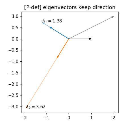
lambda is an eigenvalue of a square matrix A iff A x = lambda x for some nonzero vector x: every (lambda, x) pair returned by np.linalg.eig satisfies the defining equation, the eigenvectors are nonzero, and applying A to an eigenvector only rescales it (direction preserved — the content of the entry's figure).
print("[P-def] A x = lambda x for every eigenpair")
A = np.array([[2.0, 1.0], [1.0, 3.0]])         # symmetric -> real eigenvalues
lam, V = np.linalg.eig(A)
for i in range(2):
    x = V[:, i]
    check(f"pair {i}: ||A x - lambda x|| < 1e-12 "
          f"(lambda = {lam[i]:.4f})",
          np.linalg.norm(A @ x - lam[i] * x) < 1e-12)
    check(f"pair {i}: eigenvector is nonzero", np.linalg.norm(x) > 0)
    # direction preserved: A x is collinear with x
    cos = abs(x @ (A @ x)) / (np.linalg.norm(x) * np.linalg.norm(A @ x))
    check(f"pair {i}: A x collinear with x (|cos| = 1)",
          abs(cos - 1) < 1e-12)
# a non-eigenvector is NOT mapped to a multiple of itself
u = np.array([1.0, 0.0])
cos_u = abs(u @ (A @ u)) / (np.linalg.norm(u) * np.linalg.norm(A @ u))
check("generic vector changes direction under A (|cos| < 1)",
      cos_u < 1 - 1e-6)
[P-def] A x = lambda x for every eigenpair
  [ok] pair 0: ||A x - lambda x|| < 1e-12 (lambda = 1.3820)
  [ok] pair 0: eigenvector is nonzero
  [ok] pair 0: A x collinear with x (|cos| = 1)
  [ok] pair 1: ||A x - lambda x|| < 1e-12 (lambda = 3.6180)
  [ok] pair 1: eigenvector is nonzero
  [ok] pair 1: A x collinear with x (|cos| = 1)
  [ok] generic vector changes direction under A (|cos| < 1)
eigenvalues decide convergence of iterative methods that repeatedly apply an affine update w -> M w + b, here GD for linear regression with M = I - (2 eta/m) X^T X: the error norm is bounded by rho^t times the initial error, with rho the largest eigenvalue magnitude of M; a stepsize below m/lambda_max(X^T X) gives rho < 1 and convergence, a larger one gives rho > 1 and a growing error; each eigenvalue of M is the image of an eigenvalue of X^T X under lambda -> 1 - (2 eta/m) lambda.
print("[P-conv] largest eigenvalue magnitude of the update matrix "
      "decides convergence")
m_tr, d = 40, 2
X = rng.standard_normal((m_tr, d)) * np.array([1.0, 3.0])
y_tr = X @ np.array([1.0, -2.0]) + 0.1 * rng.standard_normal(m_tr)
Q = X.T @ X
lam_Q = np.linalg.eigvalsh(Q)
w_hat = np.linalg.solve(Q, X.T @ y_tr)


def run_gd(eta, n_iter):
    M = np.eye(d) - (2 * eta / m_tr) * Q       # affine update w -> M w + b
    b = (2 * eta / m_tr) * (X.T @ y_tr)
    rho = np.max(np.abs(np.linalg.eigvalsh(M)))
    w = np.zeros(d)
    errs = np.empty(n_iter)
    for t in range(n_iter):
        errs[t] = np.linalg.norm(w - w_hat)
        w = M @ w + b
    return rho, errs


eta_good = m_tr / (lam_Q[-1] + lam_Q[0])       # below m/lambda_max
rho_g, err_g = run_gd(eta_good, 300)
check("stepsize below m/lambda_max: rho < 1", rho_g < 1)
check("error norm bounded by rho^t times the initial error",
      np.all(err_g[:20] <= rho_g ** np.arange(20) * err_g[0] * (1 + 1e-9)))
check("error converges to 0", err_g[-1] < 1e-8 * err_g[0])
eta_bad = 1.05 * m_tr / lam_Q[-1]              # above m/lambda_max
rho_b, err_b = run_gd(eta_bad, 300)
check("stepsize above m/lambda_max: rho > 1 and the error grows",
      rho_b > 1 and err_b[-1] > err_b[0])
lam_M = np.linalg.eigvalsh(np.eye(d) - (2 * eta_good / m_tr) * Q)
check("eigenvalues of M are 1 - (2 eta/m) lambda for eigenvalues "
      "lambda of X^T X",
      np.allclose(np.sort(lam_M),
                  np.sort(1 - (2 * eta_good / m_tr) * lam_Q)))
[P-conv] largest eigenvalue magnitude of the update matrix decides convergence
  [ok] stepsize below m/lambda_max: rho < 1
  [ok] error norm bounded by rho^t times the initial error
  [ok] error converges to 0
  [ok] stepsize above m/lambda_max: rho > 1 and the error grows
  [ok] eigenvalues of M are 1 - (2 eta/m) lambda for eigenvalues lambda of X^T X
the second-smallest eigenvalue lambda_2 of a graph Laplacian measures connectivity, growing as edges are added to the same six nodes (the entry's figure): lambda_1 = 0 always; lambda_2 = 0 for two separate clusters, lambda_2 ~ 0.44 once a connecting edge is added, and lambda_2 = 6 for the complete graph; the signs of the entries of the eigenvector for lambda_2 (the Fiedler vector) recover the two clusters — spectral clustering.
print("[P-graph] second-smallest Laplacian eigenvalue measures connectivity")


def laplacian(edge_list, n):
    L = np.zeros((n, n))
    for i, j in edge_list:
        L[i, j] -= 1.0
        L[j, i] -= 1.0
        L[i, i] += 1.0
        L[j, j] += 1.0
    return L


n_nodes = 6
# two clusters of three nodes each, every pair inside a cluster linked
two_clusters = [(0, 1), (1, 2), (0, 2), (3, 4), (4, 5), (3, 5)]
with_bridge = two_clusters + [(2, 3)]          # one edge between the clusters
complete = [(i, j) for i in range(n_nodes)     # every pair of nodes linked
            for j in range(i + 1, n_nodes)]
lam_disc = np.linalg.eigvalsh(laplacian(two_clusters, n_nodes))
lam_conn, V_conn = np.linalg.eigh(laplacian(with_bridge, n_nodes))
lam_comp = np.linalg.eigvalsh(laplacian(complete, n_nodes))
check("smallest eigenvalue lambda_1 = 0 for all three graphs",
      abs(lam_disc[0]) < 1e-12 and abs(lam_conn[0]) < 1e-12
      and abs(lam_comp[0]) < 1e-12)
check("disconnected graph (no edge between clusters): lambda_2 = 0",
      abs(lam_disc[1]) < 1e-12)
check("connected graph (one edge between clusters): lambda_2 ~ 0.44",
      lam_conn[1] > 1e-8 and abs(lam_conn[1] - 0.4384) < 1e-3)
check("complete graph: lambda_2 = 6, the largest possible value",
      np.isclose(lam_comp[1], n_nodes))
fiedler = V_conn[:, 1]
side = fiedler > 0
check("signs of the Fiedler vector recover the two clusters",
      len(set(side[:3])) == 1 and len(set(side[3:])) == 1
      and side[0] != side[3])

# ------------------------------------------------------------ preview
fig, ax = plt.subplots(1, 3, figsize=(12.6, 4.0))
for i, c in zip(range(2), ("C0", "C1")):
    x = V[:, i]
    ax[0].arrow(0, 0, *x, head_width=0.06, color=c,
                length_includes_head=True)
    ax[0].arrow(0, 0, *(A @ x), head_width=0.06, color=c, alpha=0.4,
                length_includes_head=True)
    ax[0].annotate(f"$\\lambda_{i+1}={lam[i]:.2f}$", xy=A @ x)
ax[0].arrow(0, 0, *u, head_width=0.06, color="k", length_includes_head=True)
ax[0].arrow(0, 0, *(A @ u), head_width=0.06, color="k", alpha=0.35,
            length_includes_head=True)
ax[0].set_aspect("equal")
ax[0].set_xlabel("$x_1$")
ax[0].set_ylabel("$x_2$")
ax[0].set_title("[P-def] eigenvectors keep direction")
t_show = np.arange(40)
ax[1].semilogy(t_show, err_g[:40], "o-", ms=3,
               label=f"$\\rho = {rho_g:.2f} < 1$")
ax[1].semilogy(t_show, rho_g ** t_show * err_g[0], "k--",
               label="$\\rho^t \\cdot$ initial error")
ax[1].semilogy(t_show, err_b[:40], "s:", ms=3,
               label=f"$\\rho = {rho_b:.2f} > 1$")
ax[1].set_xlabel("iteration $t$")
ax[1].set_ylabel("error norm")
ax[1].set_title("[P-conv] update-matrix eigenvalues")
ax[1].legend(frameon=False)
idx = np.arange(1, n_nodes + 1)
ax[2].bar(idx - 0.26, lam_disc, width=0.24, color="C0", hatch="//",
          label="two clusters")
ax[2].bar(idx, lam_conn, width=0.24, color="C1",
          label="one connecting edge")
ax[2].bar(idx + 0.26, lam_comp, width=0.24, color="C2", hatch="xx",
          label="complete graph")
ax[2].set_xlabel("eigenvalue index $i$")
ax[2].set_ylabel("Laplacian eigenvalue $\\lambda_i$")
ax[2].set_title("[P-graph] $\\lambda_2$ grows with connectivity")
ax[2].legend(frameon=False)
fig.tight_layout()
fig.savefig(OUT_DIR / "eigenvalue.png", dpi=110)
print(f"\n{sum(ok for _, ok in report)}/{len(report)} checks passed")
assert all(ok for _, ok in report)
[P-graph] second-smallest Laplacian eigenvalue measures connectivity
  [ok] smallest eigenvalue lambda_1 = 0 for all three graphs
  [ok] disconnected graph (no edge between clusters): lambda_2 = 0
  [ok] connected graph (one edge between clusters): lambda_2 ~ 0.44
  [ok] complete graph: lambda_2 = 6, the largest possible value
  [ok] signs of the Fiedler vector recover the two clusters

17/17 checks passed
P-graph writes when the script runs