B-rp writes when the script runsDictionary of Applied Machine Learning · dimensionality reduction
Numerical companion to the entry dimensionality reduction: it recomputes what the entry states and prints one line per check
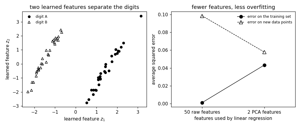
Checks the three benefits the entry attributes to using fewer features, on synthetic image-like data: the statistical benefit (less overfitting of linear regression on the learned features than on the raw ones), the computational benefit (the matrix that linear regression inverts shrinks with the number of features), and visualization (two learned features place the data points of two digits in separate regions of a scatterplot). It also checks that a random projection approximately preserves distances. Self-contained (numpy and matplotlib only), fixed seed.
Run it without installing anything:uv run https://dictionaryofml.org/terms/dimred.py
uv downloads this script and the pinned NumPy and Matplotlib it needs, then runs it; the script fetches any input file it uses. To keep the output files, download dimred.py into a folder and run uv run dimred.py there. With NumPy and Matplotlib already installed, python3 dimred.py, from any directory — it writes its output files into the current directory. Fixed seeds, so the printed numbers reproduce exactly. Download dimred.py · Notebook · Open in Colab
One cell per block of the script: the code, and what that code printed when it last ran here
"""
dimred.py — numerical companion to the glossary entry 'dimensionality
reduction'.

Purpose
-------
Checks the three benefits the entry attributes to using fewer features,
on synthetic image-like data: the statistical benefit (less overfitting
of linear regression on the learned features than on the raw ones), the
computational benefit (the matrix that linear regression inverts shrinks
with the number of features), and visualization (two learned features
place the data points of two digits in separate regions of a
scatterplot).  It also checks that a random projection approximately
preserves distances.  Self-contained (numpy and matplotlib only), fixed
seed.

Setup
-----
Each data point is a vector of d = 50 grayscale values: one of two digit
templates, which differ along one direction, plus a random variation
along two further directions plus pixel noise.  The label is a linear
function of the two variation coordinates plus noise.  Training set
m = 60 data points, and 400 further data points to measure the error on
new data points.  The
learned transformation is PCA with d' = 2 features; the random projection
uses d' = 20 features and a matrix of independent Gaussian entries.

Blocks
------
[B-pca]   PCA with d' = 2 reconstructs the raw features with an average
          squared reconstruction error below 20 percent of their total
          variance, since the data vary mainly along the digit direction
          and the larger of the two variation directions.
[B-stat]  Linear regression on the d = 50 raw features reaches an error
          near zero on the training set but an error more than ten times
          larger on new data points; on the two PCA features the error on
          new data points is less than twice the error on the training
          set and smaller than with the raw features.
[B-comp]  The matrix inverted by linear regression has 50 x 50 entries
          with the raw features and 2 x 2 with the PCA features.
[B-vis]   In the scatterplot of the two PCA features, the data points of
          the two digits occupy regions whose centers are far apart
          relative to the spread within each digit.
[B-rp]    A random projection to d' = 20 features changes every pairwise
          distance between the 60 training data points by less than a
          factor of two, and the average distance by less than 15 percent.

Outputs
-------
dimred_scatter.csv : z1, z2, digit for the 60 training data points.
dimred_errors.csv  : features, err_train, err_new for the raw and the
                     PCA features.
dimred.png         : matplotlib preview (checking only).
"""

import numpy as np
import matplotlib

matplotlib.use("Agg")
import matplotlib.pyplot as plt

from pathlib import Path

OUT_DIR = Path(__file__).parent

report = []


def check(name, ok):
    report.append((name, bool(ok)))
    print(f"  [{'ok' if ok else 'FAIL'}] {name}")


rng = np.random.default_rng(0)

d, d_pca, d_rp = 50, 2, 20
m_tr, m_va = 60, 400
templates = rng.uniform(0.0, 1.0, (2, d))          # two digit templates
Q = np.linalg.qr(rng.standard_normal((d, 3)))[0]     # three directions at right angles
directions = Q[:, :2]                                # two variation directions
templates[1] = templates[0] + 3.0 * Q[:, 2]          # digits differ along the third


def make(m):
    digit = rng.integers(0, 2, m)
    coords = rng.standard_normal((m, 2)) * np.array([1.5, 0.4])
    X = templates[digit] + coords @ directions.T + 0.1 * rng.standard_normal((m, d))
    y = 1.0 * coords[:, 0] - 0.5 * coords[:, 1] + 0.1 * rng.standard_normal(m)
    return X, y, digit


X_tr, y_tr, dig_tr = make(m_tr)
X_va, y_va, dig_va = make(m_va)
PCA with d' = 2 reconstructs the raw features with an average squared reconstruction error below 20 percent of their total variance, since the data vary mainly along the digit direction and the larger of the two variation directions.
mu = X_tr.mean(axis=0)
C = (X_tr - mu).T @ (X_tr - mu) / m_tr
evals, evecs = np.linalg.eigh(C)
W = evecs[:, ::-1][:, :d_pca]                        # d x d' transformation
Z_tr = (X_tr - mu) @ W; Z_va = (X_va - mu) @ W
recon = mu + Z_tr @ W.T
rec_err = float(np.mean(np.sum((X_tr - recon) ** 2, axis=1)))
total_var = float(np.trace(C))
check(f"[B-pca]   average squared reconstruction error {rec_err:.3f} = "
      f"{100 * rec_err / total_var:.1f} percent of the total variance "
      f"{total_var:.3f}", rec_err / total_var < 0.2)
[ok] [B-pca] average squared reconstruction error 0.610 = 12.5 percent of the total variance 4.860
Linear regression on the d = 50 raw features reaches an error near zero on the training set but an error more than ten times larger on new data points; on the two PCA features the error on new data points is less than twice the error on the training set and smaller than with the raw features.
def linreg(Xa, ya, Xb, yb):
    A = np.c_[Xa, np.ones(len(Xa))]; B = np.c_[Xb, np.ones(len(Xb))]
    w = np.linalg.lstsq(A, ya, rcond=None)[0]
    return float(np.mean((ya - A @ w) ** 2)), float(np.mean((yb - B @ w) ** 2))


tr_raw, va_raw = linreg(X_tr, y_tr, X_va, y_va)
tr_pca, va_pca = linreg(Z_tr, y_tr, Z_va, y_va)
check(f"[B-stat]  raw features: error {tr_raw:.4f} on the training set, "
      f"{va_raw:.3f} on new data points; PCA features: {tr_pca:.4f} and {va_pca:.4f}",
      va_raw > 10 * tr_raw and va_pca < 2 * tr_pca and va_pca < va_raw)
[ok] [B-stat] raw features: error 0.0013 on the training set, 0.098 on new data points; PCA features: 0.0433 and 0.0579
The matrix inverted by linear regression has 50 x 50 entries with the raw features and 2 x 2 with the PCA features.
size_raw = (X_tr.T @ X_tr).shape; size_pca = (Z_tr.T @ Z_tr).shape
check(f"[B-comp]  matrix to invert: {size_raw[0]} x {size_raw[1]} entries "
      f"with raw features, {size_pca[0]} x {size_pca[1]} with PCA features",
      size_raw == (d, d) and size_pca == (d_pca, d_pca))
[ok] [B-comp] matrix to invert: 50 x 50 entries with raw features, 2 x 2 with PCA features
In the scatterplot of the two PCA features, the data points of the two digits occupy regions whose centers are far apart relative to the spread within each digit.
c0, c1 = Z_tr[dig_tr == 0].mean(axis=0), Z_tr[dig_tr == 1].mean(axis=0)
u = (c1 - c0) / np.linalg.norm(c1 - c0)             # direction between the centers
spread = max(((Z_tr[dig_tr == 0] - c0) @ u).std(), ((Z_tr[dig_tr == 1] - c1) @ u).std())
sep = float(np.linalg.norm(c0 - c1))
check(f"[B-vis]   centers of the two digits {sep:.2f} apart in the "
      f"scatterplot, spread of a digit along that direction at most {spread:.2f}",
      sep > 3 * spread)
[ok] [B-vis] centers of the two digits 3.02 apart in the scatterplot, spread of a digit along that direction at most 0.15
A random projection to d' = 20 features changes every pairwise distance between the 60 training data points by less than a factor of two, and the average distance by less than 15 percent.
R = rng.standard_normal((d, d_rp)) / np.sqrt(d_rp)
P_tr = X_tr @ R


def pairwise(A):
    diff = A[:, None, :] - A[None, :, :]
    return np.sqrt((diff ** 2).sum(axis=2))[np.triu_indices(len(A), 1)]


ratio = pairwise(P_tr) / pairwise(X_tr)
check(f"[B-rp]    random projection to {d_rp} features: distance ratios "
      f"in [{ratio.min():.2f}, {ratio.max():.2f}], mean {ratio.mean():.3f}",
      ratio.min() > 0.5 and ratio.max() < 2.0 and abs(ratio.mean() - 1) < 0.15)

# ---------------------------------------------------------------- CSV
with open(OUT_DIR / "dimred_scatter.csv", "w") as fh:
    fh.write("z1,z2,digit\n")
    for z, g in zip(Z_tr, dig_tr):
        fh.write(f"{z[0]:.4f},{z[1]:.4f},{g}\n")
with open(OUT_DIR / "dimred_errors.csv", "w") as fh:
    fh.write("features,nfeatures,err_train,err_new\n")
    fh.write(f"raw,{d},{tr_raw:.4f},{va_raw:.4f}\n")
    fh.write(f"pca,{d_pca},{tr_pca:.4f},{va_pca:.4f}\n")

# -------------------------------------------------------------- preview
fig, (ax1, ax2) = plt.subplots(1, 2, figsize=(9.2, 3.9))
for g, mk, lab in ((0, "o", "digit A"), (1, "^", "digit B")):
    sel = dig_tr == g
    ax1.plot(Z_tr[sel, 0], Z_tr[sel, 1], mk, color="k", mfc="k" if g == 0 else "none",
             ms=5, label=lab)
ax1.set_xlabel("learned feature $z_1$"); ax1.set_ylabel("learned feature $z_2$")
ax1.set_title("two learned features separate the digits")
ax1.legend(frameon=False, fontsize=8)
xs = np.arange(2)
ax2.plot(xs, [tr_raw, tr_pca], "ko-", ms=7, lw=1.0, label="error on the training set")
ax2.plot(xs, [va_raw, va_pca], "k^--", mfc="none", ms=8, lw=1.0,
         label="error on new data points")
ax2.set_xticks(xs); ax2.set_xticklabels([f"{d} raw features", f"{d_pca} PCA features"])
ax2.set_xlim(-0.5, 1.5)
ax2.set_ylabel("average squared error"); ax2.set_xlabel("features used by linear regression")
ax2.set_title("fewer features, less overfitting")
ax2.legend(frameon=False, fontsize=8)
fig.tight_layout()
fig.savefig(OUT_DIR / "dimred.png", dpi=110)

n_ok = sum(ok for _, ok in report)
print(f"\n{n_ok}/{len(report)} checks pass")
print(f"wrote {OUT_DIR / 'dimred_scatter.csv'}, {OUT_DIR / 'dimred_errors.csv'}, "
      f"{OUT_DIR / 'dimred.png'}")
if n_ok != len(report):
    raise SystemExit(1)
  [ok] [B-rp]    random projection to 20 features: distance ratios in [0.57, 1.35], mean 0.988

5/5 checks pass
wrote /Users/junga1/dictionaryappliedml/pythondemos/dimred_scatter.csv, /Users/junga1/dictionaryappliedml/pythondemos/dimred_errors.csv, /Users/junga1/dictionaryappliedml/pythondemos/dimred.png
B-rp writes when the script runs