B-imbalance writes when the script runsDictionary of Applied Machine Learning · binary classification
Numerical companion to the entry binary classification: it recomputes what the entry states and prints one line per check
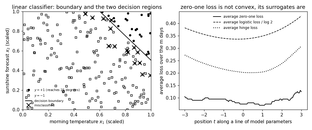
Backs the entry's claims numerically: the average zero-one loss of a classifier is 1 minus its accuracy; the decision boundary of a linear classifier is a straight line that cuts the feature space into the two decision regions; the zero-one loss is not convex in the model parameters, while the logistic loss (divided by log 2) and the hinge loss are convex and upper bound it; on imbalanced data the constant answer already has a high accuracy, so the confusion matrix with precision and recall says more than the accuracy alone. Self-contained (numpy and matplotlib only), fixed seed.
Run it without installing anything:uv run https://dictionaryofml.org/terms/binclass.py
uv downloads this script and the pinned NumPy and Matplotlib it needs, then runs it; the script fetches any input file it uses. To keep the output files, download binclass.py into a folder and run uv run binclass.py there. With NumPy and Matplotlib already installed, python3 binclass.py, from any directory — it writes its output files into the current directory. Fixed seeds, so the printed numbers reproduce exactly. Download binclass.py · Notebook · Open in Colab
One cell per block of the script: the code, and what that code printed when it last ran here
"""
binclass.py — numerical companion to the glossary entry 'binary
classification'.

Purpose
-------
Backs the entry's claims numerically: the average zero-one loss of a
classifier is 1 minus its accuracy; the decision boundary of a linear
classifier is a straight line that cuts the feature space into the two
decision regions; the zero-one loss is not convex in the model
parameters, while the logistic loss (divided by log 2) and the hinge loss
are convex and upper bound it; on imbalanced data the constant answer
already has a high accuracy, so the confusion matrix with precision and
recall says more than the accuracy alone.  Self-contained (numpy and
matplotlib only), fixed seed.

Setup
-----
The weather service of the entry: for m = 200 days, two features (the
morning temperature and the hours of sunshine forecast, both scaled to
[0, 1]) and the label y = +1 if the maximum temperature of the day
reaches 25 degrees Celsius, y = -1 otherwise.  The labels are imbalanced:
about 20 percent of the days are +1.  A linear classifier
h(x) = w^T x + b is obtained by logistic regression, i.e. by minimizing
the average logistic loss (300 small steps against its slope).

Blocks
------
[B-zeroone]   The average zero-one loss of the learned classifier equals
              1 minus its accuracy on the m days.
[B-boundary]  Every day on the +1 side of the line w^T x + b = 0 is
              predicted +1 and every day on the other side -1: the
              decision regions are the two half-planes.
[B-convex]    Along a straight line through the model parameters, the
              average zero-one loss is piecewise constant and not convex
              (it violates the midpoint inequality), while the average
              logistic loss / log 2 and the average hinge loss satisfy it
              and lie on or above the zero-one loss at every point.
[B-imbalance] The constant answer "no" reaches an accuracy of about 0.8
              with recall 0; the learned classifier's confusion matrix
              gives a recall at least 0.2 below its accuracy, a gap the
              accuracy alone hides.

Outputs
-------
binclass_data.csv : x1, x2, y of the m days and the predicted label.
binclass_line.csv : t, average zero-one, logistic / log 2 and hinge loss
                    along the line of model parameters w(t) = w_hat + t * d.
binclass_cm.csv   : the confusion matrix of the learned classifier and of
                    the constant answer, with accuracy, precision, recall.
binclass.png      : matplotlib preview of both panels (checking only).
"""

import numpy as np
import matplotlib

matplotlib.use("Agg")
import matplotlib.pyplot as plt

from pathlib import Path

OUT_DIR = Path(__file__).parent

report = []


def check(name, ok):
    report.append((name, bool(ok)))
    print(f"  [{'ok' if ok else 'FAIL'}] {name}")


rng = np.random.default_rng(0)
LOG2 = np.log(2.0)

m = 200
X = rng.uniform(0.0, 1.0, (m, 2))
score = 1.6 * X[:, 0] + 1.0 * X[:, 1] - 1.9 + 0.12 * rng.standard_normal(m)
y = np.where(score > 0, 1.0, -1.0)
Xb = np.c_[X, np.ones(m)]                       # (x1, x2, 1): w and b in one


def avg_losses(w):
    margin = y * (Xb @ w)
    return (float(np.mean(margin <= 0)),
            float(np.mean(np.log1p(np.exp(-margin))) / LOG2),
            float(np.mean(np.maximum(0.0, 1.0 - margin))))


# logistic regression: minimize the average logistic loss
w = np.zeros(3)
for _ in range(300):
    margin = y * (Xb @ w)
    slope = -(Xb * (y / (1.0 + np.exp(margin)))[:, None]).mean(axis=0)
    w = w - 1.0 * slope
y_hat = np.where(Xb @ w > 0, 1.0, -1.0)
The average zero-one loss of the learned classifier equals 1 minus its accuracy on the m days.
zo = float(np.mean(y_hat != y))
acc = float(np.mean(y_hat == y))
check(f"[B-zeroone]   average zero-one loss {zo:.3f} = 1 - accuracy "
      f"{1 - acc:.3f}", abs(zo - (1 - acc)) < 1e-12)
[ok] [B-zeroone] average zero-one loss 0.075 = 1 - accuracy 0.075
Every day on the +1 side of the line w^T x + b = 0 is predicted +1 and every day on the other side -1: the decision regions are the two half-planes.
side = np.sign(Xb @ w)
check(f"[B-boundary]  predicted label equals the side of the line "
      f"w^T x + b = 0 for all {m} days; {int(np.sum(y_hat == 1))} days "
      f"on the +1 side", np.array_equal(side, y_hat))
[ok] [B-boundary] predicted label equals the side of the line w^T x + b = 0 for all 200 days; 24 days on the +1 side
Along a straight line through the model parameters, the average zero-one loss is piecewise constant and not convex (it violates the midpoint inequality), while the average logistic loss / log 2 and the average hinge loss satisfy it and lie on or above the zero-one loss at every point.
d = np.array([1.0, -1.5, 0.4]); d /= np.linalg.norm(d)
ts = np.linspace(-3.0, 3.0, 121)
line = np.array([avg_losses(w + t * d) for t in ts])
zo_l, lg_l, hg_l = line[:, 0], line[:, 1], line[:, 2]


def midpoint_violations(v):
    # f((a+b)/2) <= (f(a)+f(b))/2 for all grid pairs a < b of equal spacing
    n = len(v); bad = 0; tot = 0
    for i in range(n):
        for j in range(i + 2, n, 2):
            k = (i + j) // 2; tot += 1
            if v[k] > (v[i] + v[j]) / 2 + 1e-9:
                bad += 1
    return bad, tot


zo_bad, tot = midpoint_violations(zo_l)
lg_bad, _ = midpoint_violations(lg_l)
hg_bad, _ = midpoint_violations(hg_l)
levels = len(np.unique(np.round(zo_l, 6)))
check(f"[B-convex]    along the line of model parameters the zero-one loss takes "
      f"{levels} values and violates the midpoint inequality {zo_bad} of "
      f"{tot} times; logistic/log 2: {lg_bad}, hinge: {hg_bad}; both "
      f"surrogates >= zero-one loss everywhere",
      zo_bad > 0 and lg_bad == 0 and hg_bad == 0
      and (lg_l >= zo_l - 1e-12).all() and (hg_l >= zo_l - 1e-12).all())
[ok] [B-convex] along the line of model parameters the zero-one loss takes 13 values and violates the midpoint inequality 1129 of 3600 times; logistic/log 2: 0, hinge: 0; both surrogates >= zero-one loss everywhere
The constant answer "no" reaches an accuracy of about 0.8 with recall 0; the learned classifier's confusion matrix gives a recall at least 0.2 below its accuracy, a gap the accuracy alone hides.
def confusion(pred):
    tp = int(np.sum((pred == 1) & (y == 1))); fn = int(np.sum((pred == -1) & (y == 1)))
    fp = int(np.sum((pred == 1) & (y == -1))); tn = int(np.sum((pred == -1) & (y == -1)))
    accuracy = (tp + tn) / m
    precision = tp / (tp + fp) if tp + fp else 0.0
    recall = tp / (tp + fn) if tp + fn else 0.0
    return tp, fn, fp, tn, accuracy, precision, recall


cm_learned = confusion(y_hat)
cm_const = confusion(-np.ones(m))
frac_pos = float(np.mean(y == 1))
check(f"[B-imbalance] {frac_pos:.2f} of the days are +1; the constant "
      f"answer -1 has accuracy {cm_const[4]:.2f} and recall "
      f"{cm_const[6]:.2f}; the learned classifier has accuracy "
      f"{cm_learned[4]:.2f}, precision {cm_learned[5]:.2f}, recall "
      f"{cm_learned[6]:.2f}",
      0.15 <= frac_pos <= 0.25 and cm_const[4] >= 0.75 and cm_const[6] == 0
      and 0.5 < cm_learned[6] < cm_learned[4] - 0.2)

# ---------------------------------------------------------------- CSV
with open(OUT_DIR / "binclass_data.csv", "w") as fh:
    fh.write("x1,x2,y,yhat\n")
    for a, b, c, e in zip(X[:, 0], X[:, 1], y, y_hat):
        fh.write(f"{a:.4f},{b:.4f},{int(c)},{int(e)}\n")
with open(OUT_DIR / "binclass_line.csv", "w") as fh:
    fh.write("t,zeroone,logistic_rescaled,hinge\n")
    for t, a, b, c in zip(ts, zo_l, lg_l, hg_l):
        fh.write(f"{t:.3f},{a:.4f},{b:.4f},{c:.4f}\n")
with open(OUT_DIR / "binclass_cm.csv", "w") as fh:
    fh.write("classifier,tp,fn,fp,tn,accuracy,precision,recall\n")
    for name, cm in (("learned", cm_learned), ("constant_no", cm_const)):
        fh.write(f"{name},{cm[0]},{cm[1]},{cm[2]},{cm[3]},{cm[4]:.4f},"
                 f"{cm[5]:.4f},{cm[6]:.4f}\n")

# -------------------------------------------------------------- preview
fig, (ax1, ax2) = plt.subplots(1, 2, figsize=(9.6, 4.0))
pos, neg = y == 1, y == -1
ax1.plot(X[pos, 0], X[pos, 1], "ko", ms=4, label="$y = +1$ (reaches 25 degrees)")
ax1.plot(X[neg, 0], X[neg, 1], "ks", mfc="none", ms=4, label="$y = -1$")
xx = np.linspace(0.0, 1.0, 50)
ax1.plot(xx, -(w[0] * xx + w[2]) / w[1], "k-", lw=1.4, label="decision boundary")
wrong = y_hat != y
ax1.plot(X[wrong, 0], X[wrong, 1], "kx", ms=9, mew=1.5, label="misclassified")
ax1.set_xlim(0, 1); ax1.set_ylim(0, 1)
ax1.set_xlabel("morning temperature $x_1$ (scaled)")
ax1.set_ylabel("sunshine forecast $x_2$ (scaled)")
ax1.set_title("linear classifier: boundary and the two decision regions")
ax1.legend(frameon=False, fontsize=7, loc="lower left")
ax2.plot(ts, zo_l, "k-", lw=1.4, label="average zero-one loss")
ax2.plot(ts, lg_l, "k--", lw=1.2, label="average logistic loss / log 2")
ax2.plot(ts, hg_l, "k:", lw=1.6, label="average hinge loss")
ax2.set_xlabel("position $t$ along a line of model parameters")
ax2.set_ylabel("average loss over the m days")
ax2.set_title("zero-one loss is not convex, its surrogates are")
ax2.legend(frameon=False, fontsize=8)
fig.tight_layout()
fig.savefig(OUT_DIR / "binclass.png", dpi=110)

n_ok = sum(ok for _, ok in report)
print(f"\n{n_ok}/{len(report)} checks pass")
print(f"wrote {OUT_DIR / 'binclass_data.csv'}, {OUT_DIR / 'binclass_line.csv'}, "
      f"{OUT_DIR / 'binclass_cm.csv'}, {OUT_DIR / 'binclass.png'}")
if n_ok != len(report):
    raise SystemExit(1)
  [ok] [B-imbalance] 0.18 of the days are +1; the constant answer -1 has accuracy 0.81 and recall 0.00; the learned classifier has accuracy 0.93, precision 0.96, recall 0.62

4/4 checks pass
wrote /Users/junga1/dictionaryappliedml/pythondemos/binclass_data.csv, /Users/junga1/dictionaryappliedml/pythondemos/binclass_line.csv, /Users/junga1/dictionaryappliedml/pythondemos/binclass_cm.csv, /Users/junga1/dictionaryappliedml/pythondemos/binclass.png
B-imbalance writes when the script runs