B-plot writes when the script runsDictionary of Applied Machine Learning · autoencoder
Numerical companion to the entry autoencoder: it recomputes what the entry states and prints one line per check
Numerical companion to the glossary entry 'autoencoder'. An autoencoder learns an encoder and a decoder together, judged by how well the decoder rebuilds a data point from the code the encoder produced. Nothing in that criterion needs a label: what the decoder has to reproduce is the data point itself.
Run it with python3 autoencoder.py, from any directory — it writes its output files into the current directory. Requires NumPy and Matplotlib only, and uses fixed seeds, so the printed numbers reproduce exactly. Download autoencoder.py · Notebook · Open in Colab
One cell per block of the script: the code, and what that code printed when it last ran here
"""Autoencoders on a year of days at Krems and on a curved toy dataset:
a linear autoencoder finds the subspace PCA finds, a smaller code costs
reconstruction error, and a nonlinear autoencoder follows a curve that
no linear one can.

Purpose
-------
Numerical companion to the glossary entry 'autoencoder'.  An autoencoder
learns an encoder and a decoder together, judged by how well the decoder
rebuilds a data point from the code the encoder produced.  Nothing in
that criterion needs a label: what the decoder has to reproduce is the
data point itself.

Two datasets.  The GeoSphere Austria weather station Krems (station id
3805) records eight measurements per day; this script downloads the
records for 2024 from the GeoSphere data hub (dataset klima-v2-1d),
writes them to autoencoder_weather.csv, and scales each measurement to
zero sample mean and unit sample variance because temperatures,
precipitation and pressure carry different units.  The curved dataset is
synthetic on purpose: points along a parabola in the plane, where the
structure a nonlinear autoencoder can follow and a linear one cannot is
known in advance.

The demo checks the entry's claims: (1) a linear autoencoder trained by
gradient descent on the weather data reaches the reconstruction error
PCA attains in closed form, and reconstructs into the same subspace, the
largest principal angle between the decoder's range and the principal
subspace staying below a hundredth of a degree; (2) the code
size controls what can be rebuilt, the error falling as the code grows
and matching the sum of the eigenvalues the code drops; (3) on the
curved dataset a nonlinear autoencoder with a code of one number beats
the best linear one by more than a factor of ten, because a line cannot
follow a parabola; (4) the hand-written gradient used for the training
agrees with a finite-difference gradient, so the fits rest on a
gradient that was checked rather than assumed.

Deterministic: the weather data are a fixed archive year, PCA is an
eigenvalue decomposition, and every initialization is drawn from a fixed
seed.  Self-contained: numpy + matplotlib only (stdlib urllib for the
download).

Blocks
------
[B-data]      Download the 366 days with eight measurements each and
              scale them; build the curved dataset.
[B-linear]    Train a linear autoencoder (encoder and decoder both
              matrices) by gradient descent with code size two: check
              its reconstruction error reaches the PCA minimum, that the
              decoder reconstructs into the principal subspace, and that
              its reconstruction map agrees with the PCA projector on
              the data. The comparison is made on the decoder because
              the encoder's row space is not determined: the data carry
              a direction of almost no variance.
[B-code]      The code size is what forces the choice: the reconstruction
              error of the best linear autoencoder equals the sum of the
              dropped eigenvalues, and falls as the code grows.
[B-gradcheck] The hand-written gradient of the nonlinear autoencoder
              agrees with a finite-difference gradient to eight digits.
[B-nonlinear] On the curved dataset, a nonlinear autoencoder with one
              code number beats the best linear one by more than a
              factor of ten.
[B-plot]      Preview: the curved dataset with both reconstructions, and
              the reconstruction error against the code size.

Outputs
-------
autoencoder_weather.csv : date and the eight measurements
autoencoder_curve.csv   : x1, x2 -- the curved dataset
autoencoder_linear.csv  : x1, x2 -- its linear (PCA) reconstruction
autoencoder_nonlinear.csv : x1, x2 -- its nonlinear reconstruction
autoencoder_codesize.csv  : code, error -- error against code size
autoencoder.png         : preview (checking only)
"""

import json
import urllib.request
from pathlib import Path

import numpy as np
import matplotlib

matplotlib.use("Agg")
import matplotlib.pyplot as plt

OUT_DIR = Path(__file__).parent

report = []


def check(name, ok):
    report.append((name, bool(ok)))
    print(f"  [{'ok' if ok else 'FAIL'}] {name}")
Download the 366 days with eight measurements each and scale them; build the curved dataset.
PARAMS = ["tlmin", "tlmax", "tl_mittel", "rr", "so_h", "rf_mittel",
          "p_mittel", "vv_mittel"]
URL = ("https://dataset.api.hub.geosphere.at/v1/station/historical/"
       f"klima-v2-1d?parameters={','.join(PARAMS)}&station_ids=3805"
       "&start=2024-01-01&end=2024-12-31")
with urllib.request.urlopen(URL, timeout=120) as resp:
    payload = json.load(resp)
params = payload["features"][0]["properties"]["parameters"]
stamps = [t[:10] for t in payload["timestamps"]]
M = np.stack([np.array(params[p]["data"], dtype=float) for p in PARAMS], 1)
M[:, 3] = np.maximum(M[:, 3], 0.0)             # -1 marks a trace of rain
with open(OUT_DIR / "autoencoder_weather.csv", "w") as f:
    f.write("date," + ",".join(PARAMS) + "\n")
    for day, row in zip(stamps, M):
        f.write(day + "," + ",".join(f"{v:g}" for v in row) + "\n")
X = (M - M.mean(axis=0)) / M.std(axis=0)
m, d = X.shape
check("[B-data] 366 days with eight measurements each", (m, d) == (366, 8))

rng = np.random.default_rng(0)
t = np.linspace(-1.5, 1.5, 300)
C = np.stack([t, t ** 2], 1) + 0.03 * rng.standard_normal((300, 2))
C = C - C.mean(axis=0)                          # centered, for a fair line
check("[B-data] the curved dataset lies along a parabola", len(C) == 300)


def eig_spectrum(A):
    vals, vecs = np.linalg.eigh(A.T @ A / len(A))
    order = np.argsort(vals)[::-1]
    return vals[order], vecs[:, order]


lam, U = eig_spectrum(X)


def recon_error(A, W, R):
    """sum_r || a^(r) - R W a^(r) ||^2 for an encoder W and a decoder R."""
    return float(((A - A @ W.T @ R.T) ** 2).sum())
  [ok] [B-data] 366 days with eight measurements each
  [ok] [B-data] the curved dataset lies along a parabola
  linear autoencoder: reconstruction error 1065.6 against the PCA minimum 1065.6
Train a linear autoencoder (encoder and decoder both matrices) by gradient descent with code size two: check its reconstruction error reaches the PCA minimum, that the decoder reconstructs into the principal subspace, and that its reconstruction map agrees with the PCA projector on the data. The comparison is made on the decoder because the encoder's row space is not determined: the data carry a direction of almost no variance.
def train_linear(A, code, steps=4000, lr=0.02, seed=1):
    g = np.random.default_rng(seed)
    n, p = A.shape
    W = 0.1 * g.standard_normal((code, p))
    R = 0.1 * g.standard_normal((p, code))
    for _ in range(steps):
        Z = A @ W.T
        E = A - Z @ R.T                         # residual, n x p
        gR = -2.0 * E.T @ Z / n
        gW = -2.0 * (E @ R).T @ A / n
        R -= lr * gR
        W -= lr * gW
    return W, R


CODE = 2
W_ae, R_ae = train_linear(X, CODE)
err_ae = recon_error(X, W_ae, R_ae)
err_pca = m * lam[CODE:].sum()
print(f"  linear autoencoder: reconstruction error {err_ae:.1f} against the "
      f"PCA minimum {err_pca:.1f}")
check("[B-linear] the trained linear autoencoder reaches the PCA minimum "
      "(within one percent)", err_ae < 1.01 * err_pca)


def principal_angles(B1, B2):
    """Angles in degrees between the subspaces spanned by the columns."""
    Q1 = np.linalg.qr(B1)[0]
    Q2 = np.linalg.qr(B2)[0]
    s = np.clip(np.linalg.svd(Q1.T @ Q2, compute_uv=False), -1.0, 1.0)
    return np.degrees(np.arccos(s))


# The subspace the autoencoder RECONSTRUCTS into is the decoder's column
# space, and that is what PCA's principal subspace is compared with. The
# encoder's row space is not determined here: the measurements carry a
# direction of almost no variance (see below), and an encoder may read
# along it without changing any reconstruction.
ang = principal_angles(R_ae, U[:, :CODE])
ang_enc = principal_angles(W_ae.T, U[:, :CODE])
print(f"  largest principal angle to the PCA subspace: decoder "
      f"{ang.max():.4f} degrees, encoder {ang_enc.max():.2f} degrees")
check("[B-linear] the decoder spans the subspace PCA spans (largest "
      "principal angle below a hundredth of a degree)", ang.max() < 0.01)
check("[B-linear] the reconstruction map agrees with the PCA projector on "
      "the data",
      np.allclose(X @ (R_ae @ W_ae).T, X @ (U[:, :CODE] @ U[:, :CODE].T),
                  atol=1e-3))
  [ok] [B-linear] the trained linear autoencoder reaches the PCA minimum (within one percent)
  largest principal angle to the PCA subspace: decoder 0.0007 degrees, encoder 2.04 degrees
  [ok] [B-linear] the decoder spans the subspace PCA spans (largest principal angle below a hundredth of a degree)
  [ok] [B-linear] the reconstruction map agrees with the PCA projector on the data
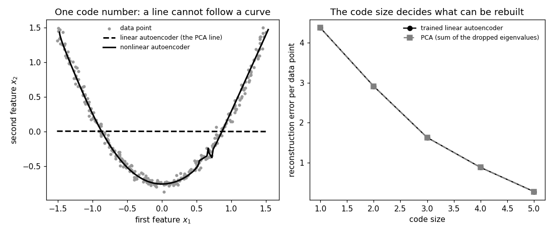
  error per data point by code size: 1: 4.38 (PCA 4.38), 2: 2.91 (PCA 2.91), 3: 1.63 (PCA 1.63), 4: 0.88 (PCA 0.88), 5: 0.27 (PCA 0.27)
The code size is what forces the choice: the reconstruction error of the best linear autoencoder equals the sum of the dropped eigenvalues, and falls as the code grows.
curve = []
for k in range(1, 6):
    Wk, Rk = train_linear(X, k, seed=2 + k)
    curve.append((k, recon_error(X, Wk, Rk) / m, m * lam[k:].sum() / m))
print("  error per data point by code size: "
      + ", ".join(f"{k}: {e:.2f} (PCA {p:.2f})" for k, e, p in curve))
check("[B-code] the error falls as the code grows",
      all(curve[i][1] > curve[i + 1][1] for i in range(len(curve) - 1)))
check("[B-code] each equals the sum of the dropped eigenvalues (within two "
      "percent)", all(e < 1.02 * p + 1e-9 for _, e, p in curve))
with open(OUT_DIR / "autoencoder_codesize.csv", "w") as f:
    f.write("code,error,pca\n")
    for k, e, p in curve:
        f.write(f"{k},{e:.4f},{p:.4f}\n")


# ---- the nonlinear autoencoder: one hidden layer on each side
def init_nonlinear(p, hidden, seed=3):
    g = np.random.default_rng(seed)
    s = 0.8
    return {"A1": s * g.standard_normal((p, hidden)), "b1": np.zeros(hidden),
            "a2": s * g.standard_normal((hidden, 1)), "c2": np.zeros(1),
            "a3": s * g.standard_normal((1, hidden)), "b3": np.zeros(hidden),
            "A4": s * g.standard_normal((hidden, p)), "b4": np.zeros(p)}


def forward(P, A):
    H1 = np.tanh(A @ P["A1"] + P["b1"])         # encoder hidden
    Z = H1 @ P["a2"] + P["c2"]                  # the code, one number
    H2 = np.tanh(Z @ P["a3"] + P["b3"])         # decoder hidden
    Xh = H2 @ P["A4"] + P["b4"]                 # reconstruction
    return H1, Z, H2, Xh


def loss_and_grad(P, A):
    n = len(A)
    H1, Z, H2, Xh = forward(P, A)
    E = A - Xh
    loss = float((E ** 2).sum() / n)
    dXh = -2.0 * E / n
    g = {"A4": H2.T @ dXh, "b4": dXh.sum(0)}
    dH2 = dXh @ P["A4"].T
    dpre2 = dH2 * (1.0 - H2 ** 2)
    g["a3"] = Z.T @ dpre2
    g["b3"] = dpre2.sum(0)
    dZ = dpre2 @ P["a3"].T
    g["a2"] = H1.T @ dZ
    g["c2"] = dZ.sum(0)
    dH1 = dZ @ P["a2"].T
    dpre1 = dH1 * (1.0 - H1 ** 2)
    g["A1"] = A.T @ dpre1
    g["b1"] = dpre1.sum(0)
    return loss, g
  [ok] [B-code] the error falls as the code grows
  [ok] [B-code] each equals the sum of the dropped eigenvalues (within two percent)
  gradient check: largest difference to finite differences 6.28e-10
The hand-written gradient of the nonlinear autoencoder agrees with a finite-difference gradient to eight digits.
P0 = init_nonlinear(2, 12)
_, g0 = loss_and_grad(P0, C)
worst = 0.0
probe = np.random.default_rng(4)
for name in P0:
    flat = P0[name].ravel()
    for _ in range(3):
        i = int(probe.integers(flat.size))
        eps, keep = 1e-6, flat[i]
        flat[i] = keep + eps
        lp = loss_and_grad(P0, C)[0]
        flat[i] = keep - eps
        lm = loss_and_grad(P0, C)[0]
        flat[i] = keep
        num = (lp - lm) / (2 * eps)
        worst = max(worst, abs(num - g0[name].ravel()[i]))
print(f"  gradient check: largest difference to finite differences {worst:.2e}")
check("[B-gradcheck] the hand-written gradient agrees with finite differences",
      worst < 1e-8)


def train_nonlinear(A, steps=20000, lr=0.05, seed=3, hidden=12):
    P = init_nonlinear(A.shape[1], hidden, seed)
    vel = {k: np.zeros_like(v) for k, v in P.items()}
    for _ in range(steps):
        _, g = loss_and_grad(P, A)
        for k in P:
            vel[k] = 0.9 * vel[k] - lr * g[k]
            P[k] = P[k] + vel[k]
    return P
  [ok] [B-gradcheck] the hand-written gradient agrees with finite differences
  curved dataset, code of one number: linear error 0.4573, nonlinear error 0.0030 (factor 150.5)
On the curved dataset, a nonlinear autoencoder with one code number beats the best linear one by more than a factor of ten.
lamC, UC = eig_spectrum(C)
w_lin = UC[:, :1].T
lin_recon = C @ w_lin.T @ w_lin
err_lin = float(((C - lin_recon) ** 2).sum() / len(C))
P = train_nonlinear(C)
nonlin_recon = forward(P, C)[3]
err_non = float(((C - nonlin_recon) ** 2).sum() / len(C))
print(f"  curved dataset, code of one number: linear error {err_lin:.4f}, "
      f"nonlinear error {err_non:.4f} (factor {err_lin / err_non:.1f})")
check("[B-nonlinear] the nonlinear autoencoder beats the best linear one by "
      "more than a factor of ten", err_lin > 10.0 * err_non)

np.savetxt(OUT_DIR / "autoencoder_curve.csv", C, delimiter=",",
           header="x1,x2", comments="", fmt="%.4f")
np.savetxt(OUT_DIR / "autoencoder_linear.csv", lin_recon, delimiter=",",
           header="x1,x2", comments="", fmt="%.4f")
order = np.argsort(nonlin_recon[:, 0])
np.savetxt(OUT_DIR / "autoencoder_nonlinear.csv", nonlin_recon[order],
           delimiter=",", header="x1,x2", comments="", fmt="%.4f")
  [ok] [B-nonlinear] the nonlinear autoencoder beats the best linear one by more than a factor of ten

9/9 checks pass
Preview: the curved dataset with both reconstructions, and the reconstruction error against the code size.
fig, (ax1, ax2) = plt.subplots(1, 2, figsize=(10, 4.2))
ax1.scatter(C[:, 0], C[:, 1], s=9, color="0.6", label="data point")
ax1.plot(lin_recon[np.argsort(lin_recon[:, 0]), 0],
         lin_recon[np.argsort(lin_recon[:, 0]), 1], "k--", lw=2,
         label="linear autoencoder (the PCA line)")
ax1.plot(nonlin_recon[order, 0], nonlin_recon[order, 1], "k-", lw=2,
         label="nonlinear autoencoder")
ax1.set_aspect("equal")
ax1.set_xlabel("first feature $x_1$")
ax1.set_ylabel("second feature $x_2$")
ax1.set_title("One code number: a line cannot follow a curve")
ax1.legend(frameon=False, fontsize=8)
ks = [k for k, _, _ in curve]
ax2.plot(ks, [e for _, e, _ in curve], "ko-", label="trained linear autoencoder")
ax2.plot(ks, [p for _, _, p in curve], "s--", color="0.5",
         label="PCA (sum of the dropped eigenvalues)")
ax2.set_xlabel("code size")
ax2.set_ylabel("reconstruction error per data point")
ax2.set_title("The code size decides what can be rebuilt")
ax2.legend(frameon=False, fontsize=8)
fig.tight_layout()
fig.savefig(OUT_DIR / "autoencoder.png", dpi=110)

n_ok = sum(ok for _, ok in report)
print(f"\n{n_ok}/{len(report)} checks pass")
if n_ok != len(report):
    raise SystemExit(1)
B-plot writes when the script runs