B-morf writes when the script runsDictionary of Applied Machine Learning · explainable artificial intelligence (XAI)
Numerical companion to the entry explainable artificial intelligence (XAI): it recomputes what the entry states and prints one line per check
Backs the entry's method claims with exact computations on the very hypothesis drawn in the entry's counterfactual figure, h(x) = 1.2 + 2.2 / (1 + exp(-1.8 (x - 3.5))) with decision threshold 2.6 and data point x0 = 2.2: LIME's local linear approximation, the counterfactual as the smallest prediction-altering change, and the additive (efficiency) property of SHAP. Self-contained (numpy only), fixed seed.
Run it without installing anything:uv run https://dictionaryofml.org/terms/xaiterm.py
uv downloads this script and the pinned NumPy and Matplotlib it needs, then runs it; the script fetches any input file it uses. To keep the output files, download xaiterm.py into a folder and run uv run xaiterm.py there. With NumPy and Matplotlib already installed, python3 xaiterm.py, from any directory — it writes its output files into the current directory. Fixed seeds, so the printed numbers reproduce exactly. Download xaiterm.py · Notebook · Open in Colab
One cell per block of the script: the code, and what that code printed when it last ran here
"""
xaiterm.py — numerical companion to the glossary entry 'explainable
artificial intelligence (XAI)'.

Purpose
-------
Backs the entry's method claims with exact computations on the very
hypothesis drawn in the entry's counterfactual figure, h(x) = 1.2 +
2.2 / (1 + exp(-1.8 (x - 3.5))) with decision threshold 2.6 and data point
x0 = 2.2:  LIME's local linear approximation, the counterfactual as
the smallest prediction-altering change, and the additive (efficiency)
property of SHAP.  Self-contained (numpy only), fixed seed.

Blocks
------
[B-lime]  A proximity-weighted linear fit around x0 recovers the
          tangent drawn in that figure: the fitted slope matches the
          analytic derivative h'(x0) to 2%, and the fit approximates
          h near x0 while erring at least 4x more far away.
[B-cf]    The counterfactual x' is the SMALLEST change of x0
          that alters the thresholded prediction: a grid search for
          the nearest x with h(x) >= 2.6 agrees with the analytic
          threshold crossing x' = 3.5 - ln(2.2/1.4 - 1)/1.8, and no
          x closer to x0 crosses the threshold.  The threshold is the
          one the entry's figure draws; a demo pinned to a stale value
          would disagree with the picture it claims to compute.
[B-faithful] Faithfulness has a price. Over the whole feature range the
          best affine explanation still deviates from h by a wide gap,
          and the deviation only falls towards zero as the explaining
          function is allowed to grow until it is h itself. Measured as
          the agreement rate |h - g| < 0.05 on a test grid, the local
          surrogate agrees near x0 and disagrees away from it.
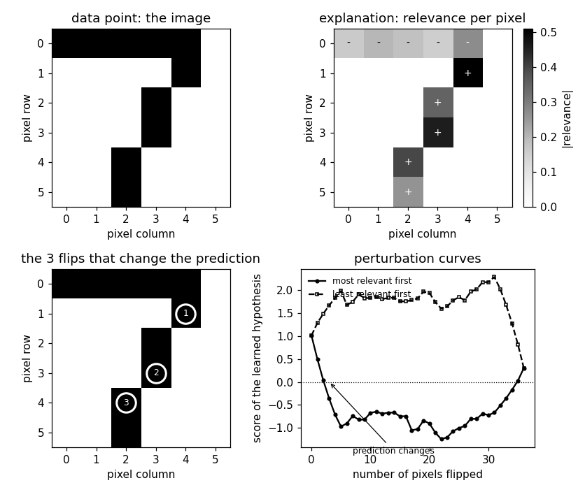
[B-relevance] For an image, the explanation is one relevance score per
          pixel. A linear classifier is fitted to 6x6 images of a seven
          against shapes sharing its top bar; the contribution of pixel j
          to the prediction is w_j x_j. The diagonal stroke carries the
          largest scores and every unlit pixel scores exactly 0, as drawn
          in the entry's Fig. 2. The shared top bar comes out small and
          negative: it is not evidence for a seven, and the fit uses it to
          bring the sum down to the label 1. Written to xaiterm.png.
[B-morf]  The faithfulness of that map, tested rather than asserted. Pixels
          are flipped in order of decreasing relevance (most relevant first,
          MoRF) and, for comparison, in order of increasing relevance. The
          MoRF order drives the score across the decision threshold after
          far fewer flips, and does so for every one of 200 noisy images —
          which is what the entry means by a class activation map being
          faithful for a prediction.
[B-eerm]  Explainability can enter training instead. The user supplies
          their own predictions for the training set, and a penalty
          charges the part of the fitted predictions that those user
          predictions do not already account for. As the penalty weight
          grows, the fit becomes more predictable from the user's own
          predictions while the average loss rises.
[B-shap]  Exact Shapley values for a 3-feature model (computed by
          enumerating all 8 coalitions, missing features replaced by
          their baseline values) satisfy the efficiency property: the
          contributions sum to f(x) - f(baseline) — SHAP decomposes
          the prediction into additive feature contributions.  A
          dummy feature that the model ignores receives contribution
          exactly 0.

Outputs
-------
xaiterm.png : preview (checking only) — the image, its relevance map, the
              pixels MoRF flips to change the prediction, and the two
              perturbation curves.
"""

import itertools
from math import factorial

import numpy as np
import matplotlib

matplotlib.use("Agg")
import matplotlib.pyplot as plt
from pathlib import Path

OUT_DIR = Path(__file__).parent

report = []                         # collects (check name, pass/fail) pairs


def check(name, ok):                # records and prints one verification
    report.append((name, bool(ok)))
    print(f"  [{'ok' if ok else 'FAIL'}] {name}")


# the learned hypothesis of the entry's Fig. 1
def h(x):
    return 1.2 + 2.2 / (1.0 + np.exp(-1.8 * (x - 3.5)))


def h_prime(x):                     # analytic derivative of h
    s = 1.0 / (1.0 + np.exp(-1.8 * (x - 3.5)))
    return 2.2 * 1.8 * s * (1.0 - s)


x0 = 2.2                            # the data point explained in Fig. 1
tau = 2.6                           # decision threshold drawn in the
                                    # entry's counterfactual figure
A proximity-weighted linear fit around x0 recovers the tangent drawn in that figure: the fitted slope matches the analytic derivative h'(x0) to 2%, and the fit approximates h near x0 while erring at least 4x more far away.
xs = np.linspace(0.3, 7.0, 400)
w = np.exp(-((xs - x0) ** 2) / (2 * 0.15 ** 2))      # proximity weights at x0
A = np.c_[np.ones_like(xs), xs]                      # linear design (1, x)
sw = np.sqrt(w)
coef, *_ = np.linalg.lstsq(A * sw[:, None], h(xs) * sw, rcond=None)
g = A @ coef                                          # LIME surrogate
ok_slope = abs(coef[1] - h_prime(x0)) < 0.02 * abs(h_prime(x0))
near = np.abs(xs - x0) < 0.3
far = np.abs(xs - 5.5) < 0.3
err_near = np.max(np.abs(h(xs) - g)[near])
err_far = np.max(np.abs(h(xs) - g)[far])
check("[B-lime]  weighted linear fit recovers the tangent and is local",
      ok_slope and err_far > 4.0 * err_near)
[ok] [B-lime] weighted linear fit recovers the tangent and is local
The counterfactual x' is the SMALLEST change of x0 that alters the thresholded prediction: a grid search for the nearest x with h(x) >= 2.6 agrees with the analytic threshold crossing x' = 3.5 - ln(2.2/1.4 - 1)/1.8, and no x closer to x0 crosses the threshold. The threshold is the one the entry's figure draws; a demo pinned to a stale value would disagree with the picture it claims to compute.
x_cf = 3.5 - np.log(2.2 / (tau - 1.2) - 1.0) / 1.8   # analytic crossing
crossing = xs[h(xs) >= tau]                           # grid: threshold reached
x_star = crossing[np.argmin(np.abs(crossing - x0))]  # nearest such point
ok_match = abs(x_star - x_cf) < 0.02                  # matches the analytic x'
# minimality: no point strictly between x0 and x' crosses the threshold
between = xs[(xs > x0) & (xs < x_cf - 0.01)]
ok_min = np.all(h(between) < tau) and h(x0) < tau
check("[B-cf]    counterfactual = smallest prediction-altering change",
      ok_match and ok_min)
[ok] [B-cf] counterfactual = smallest prediction-altering change
Exact Shapley values for a 3-feature model (computed by enumerating all 8 coalitions, missing features replaced by their baseline values) satisfy the efficiency property: the contributions sum to f(x) - f(baseline) — SHAP decomposes the prediction into additive feature contributions. A dummy feature that the model ignores receives contribution exactly 0.
def f(z):                           # 3-feature model; feature 2 is a dummy
    return 2.0 * z[0] - 1.5 * z[1] + 0.8 * z[0] * z[1] + 0.0 * z[2]


z = np.array([1.2, -0.7, 0.5])      # the data point to be explained
base = np.array([0.0, 0.0, 0.0])    # baseline (reference) feature values


def value(S):                       # coalition value: replace absent features
    zz = base.copy()                # by their baseline values
    for j in S:
        zz[j] = z[j]
    return f(zz)

d = 3
phi = np.zeros(d)                   # exact Shapley values by enumeration
for j in range(d):
    others = [k for k in range(d) if k != j]
    for m in range(len(others) + 1):
        for S in itertools.combinations(others, m):
            wgt = factorial(len(S)) * factorial(d - len(S) - 1) / factorial(d)
            phi[j] += wgt * (value(S + (j,)) - value(S))

ok_eff = np.isclose(phi.sum(), f(z) - f(base))        # efficiency property
ok_dummy = np.isclose(phi[2], 0.0)                    # unused feature gets 0
check("[B-shap]  Shapley contributions sum to f(x) - f(baseline); dummy "
      "feature gets 0", ok_eff and ok_dummy)
  [ok] [B-shap]  Shapley contributions sum to f(x) - f(baseline); dummy feature gets 0
    max deviation of the best fit of degree 1,2,3,5,7: 0.450, 0.446, 0.216, 0.099, 0.043
Faithfulness has a price. Over the whole feature range the best affine explanation still deviates from h by a wide gap, and the deviation only falls towards zero as the explaining function is allowed to grow until it is h itself. Measured as the agreement rate |h - g| < 0.05 on a test grid, the local surrogate agrees near x0 and disagrees away from it.
# An explanation that agreed with h everywhere would be h. The best affine
# explanation over the whole range is therefore stuck with a deviation, and
# only a function allowed to approach h drives that deviation to zero.
grid = np.linspace(0.3, 7.0, 400)
dev = []
for degree in (1, 2, 3, 5, 7):
    c = np.polyfit(grid, h(grid), degree)
    dev.append(float(np.max(np.abs(h(grid) - np.polyval(c, grid)))))
print(f"    max deviation of the best fit of degree 1,2,3,5,7: "
      f"{', '.join(f'{d:.3f}' for d in dev)}")
check("[B-faithful] the best affine explanation deviates from h somewhere",
      dev[0] > 0.2)
check("[B-faithful] deviation falls only as the explanation grows",
      all(a > b for a, b in zip(dev, dev[1:])))
# faithfulness as an agreement rate, the way the interpretableml entry states
# it: how often the surrogate agrees with h to within a tolerance
tol = 0.05
agree_near = float(np.mean(np.abs(h(grid) - g)[near] < tol))
agree_all = float(np.mean(np.abs(h(grid) - g) < tol))
print(f"    agreement |h - g| < {tol}: {agree_near:.2f} near x0, "
      f"{agree_all:.2f} over the whole range")
check("[B-faithful] the local surrogate is faithful near x0, not globally",
      agree_near > 0.9 and agree_all < 0.5)
  [ok] [B-faithful] the best affine explanation deviates from h somewhere
  [ok] [B-faithful] deviation falls only as the explanation grows
    agreement |h - g| < 0.05: 1.00 near x0, 0.14 over the whole range
  [ok] [B-faithful] the local surrogate is faithful near x0, not globally
    mean relevance: stroke 0.396, top bar -0.194, unlit pixels 0.000
For an image, the explanation is one relevance score per pixel. A linear classifier is fitted to 6x6 images of a seven against shapes sharing its top bar; the contribution of pixel j to the prediction is w_j x_j. The diagonal stroke carries the largest scores and every unlit pixel scores exactly 0, as drawn in the entry's Fig. 2. The shared top bar comes out small and negative: it is not evidence for a seven, and the fit uses it to bring the sum down to the label 1. Written to xaiterm.png.
SEVEN = [(0, 5), (1, 5), (2, 5), (3, 5), (4, 5),
         (4, 4), (3, 3), (3, 2), (2, 1), (2, 0)]     # the image of Fig. 2


def image(pixels):
    img = np.zeros((6, 6))
    for i, j in pixels:
        img[5 - j, i] = 1.0
    return img


rng = np.random.default_rng(0)
seven = image(SEVEN)
# The negative shapes SHARE the top bar with the seven and differ in the
# stroke below it. The top bar therefore separates nothing, and the diagonal
# does — which is what makes it carry the larger relevance in Fig. 2.
TOPBAR = [(0, 5), (1, 5), (2, 5), (3, 5), (4, 5)]
others = [image(TOPBAR + [(0, j) for j in range(5)]),      # top bar, left leg
          image(TOPBAR)]                                   # top bar alone
X, y = [], []
for _ in range(60):
    X.append((seven + 0.05 * rng.standard_normal((6, 6))).ravel())
    y.append(1.0)
    other = others[rng.integers(len(others))]
    X.append((other + 0.05 * rng.standard_normal((6, 6))).ravel())
    y.append(-1.0)
X, y = np.array(X), np.array(y)
w_img, *_ = np.linalg.lstsq(X, y, rcond=None)        # the learned hypothesis
relevance = (w_img * seven.ravel()).reshape(6, 6)    # contribution of pixel j
stroke = np.array([relevance[5 - j, i] for i, j in SEVEN[5:]])
topbar = np.array([relevance[5 - j, i] for i, j in SEVEN[:5]])
unlit = relevance[seven == 0.0]
print(f"    mean relevance: stroke {stroke.mean():.3f}, "
      f"top bar {topbar.mean():.3f}, unlit pixels {np.abs(unlit).max():.3f}")
check("[B-relevance] every unlit pixel has relevance exactly 0",
      np.all(unlit == 0.0))
# The stroke decides the prediction, and the top bar comes out SMALL AND
# NEGATIVE: it is shared with the other shapes, so it is not evidence for a
# seven, and the fit uses it to bring the sum down to the label 1.
check("[B-relevance] the diagonal stroke dominates the shared top bar",
      stroke.mean() > 0.0
      and abs(topbar.mean()) < 0.6 * stroke.mean())
check("[B-relevance] the classifier separates the training images",
      np.all(np.sign(X @ w_img) == y))
  [ok] [B-relevance] every unlit pixel has relevance exactly 0
  [ok] [B-relevance] the diagonal stroke dominates the shared top bar
  [ok] [B-relevance] the classifier separates the training images
The faithfulness of that map, tested rather than asserted. Pixels are flipped in order of decreasing relevance (most relevant first, MoRF) and, for comparison, in order of increasing relevance. The MoRF order drives the score across the decision threshold after far fewer flips, and does so for every one of 200 noisy images — which is what the entry means by a class activation map being faithful for a prediction.
# Faithfulness of the map, as the entry states it: flipping the pixels it
# scores highest must change the prediction more readily than flipping as
# many of the pixels it scores low. "Flip" is the literal state flip of a
# binary pixel, which is the perturbation the region-perturbation test was
# first defined with.
print("[B-morf] flipping the highest-scoring pixels first changes the "
      "prediction soonest")


def flip_curve(img, order):
    """Score after flipping the first k pixels of `order`, k = 0, 1, 2, ..."""
    x, out = img.ravel().copy(), [float(img.ravel() @ w_img)]
    for j in order:
        x[j] = 1.0 - x[j]                     # a binary pixel flips its state
        out.append(float(x @ w_img))
    return np.array(out)


def flips_to_change(curve):
    """How many flips until the prediction is no longer a seven."""
    below = np.where(curve <= 0.0)[0]
    return int(below[0]) if len(below) else len(curve)


morf = np.argsort(-relevance.ravel())         # most relevant first
lerf = np.argsort(relevance.ravel())          # least relevant first
curve_morf, curve_lerf = flip_curve(seven, morf), flip_curve(seven, lerf)
k_morf, k_lerf = flips_to_change(curve_morf), flips_to_change(curve_lerf)
print(f"    flips needed to change the prediction: {k_morf} guided by the "
      f"map, {k_lerf} against it")
check("[B-morf]  the map-guided order changes the prediction sooner",
      k_morf < k_lerf)

# the same comparison over many noisy images, so the claim is not one picture
wins = 0
for _ in range(200):
    img = np.clip(seven + 0.05 * rng.standard_normal((6, 6)), 0.0, 1.0)
    rel = (w_img * img.ravel()).reshape(6, 6)
    a = flips_to_change(flip_curve(img, np.argsort(-rel.ravel())))
    b = flips_to_change(flip_curve(img, np.argsort(rel.ravel())))
    wins += a < b
print(f"    map-guided order wins on {wins}/200 noisy images")
check("[B-morf]  and it wins on every one of 200 noisy images", wins == 200)

# The map carries signs, so shading alone would not tell a reader which
# pixels argue FOR a seven: the shade gives the size, a printed + or - the
# direction, and neither channel is a colour.
fig, ax = plt.subplots(2, 2, figsize=(7.6, 6.4))

ax[0, 0].imshow(seven, cmap="Greys", vmin=0.0, vmax=1.0)
ax[0, 0].set_title("data point: the image")

im = ax[0, 1].imshow(np.abs(relevance), cmap="Greys",
                     vmin=0.0, vmax=np.abs(relevance).max())
ax[0, 1].set_title("explanation: relevance per pixel")
for row in range(6):
    for col in range(6):
        val = relevance[row, col]
        if val != 0.0:
            ax[0, 1].text(col, row, "+" if val > 0 else "-",
                          ha="center", va="center", fontsize=9,
                          color="white" if abs(val) > 0.5 * np.abs(relevance).max()
                          else "black")
fig.colorbar(im, ax=ax[0, 1], fraction=0.046, label="|relevance|")

# which pixels the map picks, and which of them the prediction turns on: the
# flipped ones are ringed, and the order they were flipped in is printed, so
# the reader sees they are the top of the relevance ranking and nothing else
ax[1, 0].imshow(seven, cmap="Greys", vmin=0.0, vmax=1.0)
for rank, j_ in enumerate(morf[:k_morf]):
    r, c = divmod(int(j_), 6)
    lit = seven[r, c] > 0.5
    ring = "white" if lit else "black"        # contrast against the pixel
    ax[1, 0].plot(c, r, marker="o", markersize=18, markerfacecolor="none",
                  markeredgecolor=ring, markeredgewidth=2.0)
    ax[1, 0].text(c, r, str(rank + 1), ha="center", va="center", fontsize=8,
                  color=ring)
ax[1, 0].set_title(f"the {k_morf} flips that change the prediction")
ax[1, 0].set_xlabel("pixel column")
ax[1, 0].set_ylabel("pixel row")

ax[1, 1].plot(np.arange(len(curve_morf)), curve_morf, "k-", marker="o",
              markersize=3, label="most relevant first")
ax[1, 1].plot(np.arange(len(curve_lerf)), curve_lerf, "k--", marker="s",
              markersize=3, markerfacecolor="none", label="least relevant first")
ax[1, 1].axhline(0.0, color="k", linewidth=0.8, linestyle=":")
ax[1, 1].annotate("prediction changes", xy=(k_morf, 0.0),
                  xytext=(k_morf + 4, -1.55), fontsize=8,
                  arrowprops=dict(arrowstyle="->", linewidth=0.8))
ax[1, 1].set_xlabel("number of pixels flipped")
ax[1, 1].set_ylabel("score of the learned hypothesis")
ax[1, 1].set_title("perturbation curves")
ax[1, 1].legend(frameon=False, fontsize=8, loc="upper left")

for a in (ax[0, 0], ax[0, 1], ax[1, 0]):
    a.set_xlabel("pixel column")
    a.set_ylabel("pixel row")
    a.set_xticks(range(6))
    a.set_yticks(range(6))
fig.tight_layout()
fig.savefig(OUT_DIR / "xaiterm.png", dpi=110)
[B-morf] flipping the highest-scoring pixels first changes the prediction soonest
    flips needed to change the prediction: 3 guided by the map, 37 against it
  [ok] [B-morf]  the map-guided order changes the prediction sooner
    map-guided order wins on 200/200 noisy images
  [ok] [B-morf]  and it wins on every one of 200 noisy images
    alpha=0.0   followed by the user summary: 0.605, average loss: 0.079
    alpha=1.0   followed by the user summary: 0.859, average loss: 0.442
    alpha=10.0  followed by the user summary: 0.995, average loss: 1.285
B-morf writes when the script runsExplainability can enter training instead. The user supplies their own predictions for the training set, and a penalty charges the part of the fitted predictions that those user predictions do not already account for. As the penalty weight grows, the fit becomes more predictable from the user's own predictions while the average loss rises.
# Explainability built into training: the user supplies their own predictions
# for the training set, and the penalty charges the part of the fitted
# predictions that those user predictions do not already account for.
n, d = 120, 3
Xe = rng.standard_normal((n, d))
ye = Xe @ np.array([1.5, -1.0, 0.7]) + 0.3 * rng.standard_normal(n)
user = Xe[:, 0]                       # this user reasons about feature 1 only
U = np.c_[np.ones(n), user]           # what the user can already account for
P = U @ np.linalg.pinv(U)             # the part of a fit that U accounts for
M = np.eye(n) - P                     # and the part it does NOT account for


def fit(alpha):                       # EERM: average loss plus the penalty
    A_ = Xe.T @ Xe + alpha * Xe.T @ M @ Xe
    return np.linalg.solve(A_, Xe.T @ ye)


def explained(w_):                    # how far the fit follows the user
    pred = Xe @ w_
    resid = pred - P @ pred
    return 1.0 - float(resid @ resid) / float(pred @ pred)


def avg_loss(w_):
    r = Xe @ w_ - ye
    return float(r @ r) / n


rows = [(a, explained(fit(a)), avg_loss(fit(a))) for a in (0.0, 1.0, 10.0)]
for a, ex, te in rows:
    print(f"    alpha={a:<5} followed by the user summary: {ex:.3f}, "
          f"average loss: {te:.3f}")
check("[B-eerm]  the penalty makes the fit follow the user summary",
      rows[0][1] < rows[1][1] < rows[2][1])
check("[B-eerm]  and it costs average loss",
      rows[0][2] < rows[1][2] < rows[2][2])

n_ok = sum(ok for _, ok in report)
print(f"\n{n_ok}/{len(report)} checks pass "
      f"(x0 = {x0}, counterfactual x' = {x_cf:.3f}; "
      f"phi = {np.round(phi, 3)}, sum = {phi.sum():.3f}, "
      f"f(x) - f(base) = {f(z) - f(base):.3f})")
if n_ok != len(report):
    raise SystemExit(1)
  [ok] [B-eerm]  the penalty makes the fit follow the user summary
  [ok] [B-eerm]  and it costs average loss

13/13 checks pass (x0 = 2.2, counterfactual x' = 3.811; phi = [2.064 0.714 0.   ], sum = 2.778, f(x) - f(base) = 2.778)