B-oversight writes when the script runsDictionary of Applied Machine Learning · trustworthy artificial intelligence (trustworthy AI)
Numerical companion to the entry trustworthy artificial intelligence (trustworthy AI): it recomputes what the entry states and prints one line per check
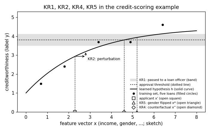
The entry locates four of the seven key requirements (KRs) for trustworthy AI in the credit-scoring example of its Fig. 1: a learned hypothesis h approves a loan when the predicted creditworthiness h(x) exceeds the threshold tau = 3.8. The figure is a cartoon drawn from the closed form h(x) = 1 + 3.5 (1 - exp(-0.35 x)) over a one-dimensional sketch of the feature vector, with a training set of five completed loans; this demo checks every number the entry states about it. Self-contained (numpy/matplotlib only), no randomness.
Run it without installing anything:uv run https://dictionaryofml.org/terms/trustAI.py
uv downloads this script and the pinned NumPy and Matplotlib it needs, then runs it; the script fetches any input file it uses. To keep the output files, download trustAI.py into a folder and run uv run trustAI.py there. With NumPy and Matplotlib already installed, python3 trustAI.py, from any directory — it writes its output files into the current directory. Fixed seeds, so the printed numbers reproduce exactly. Download trustAI.py · Notebook · Open in Colab
One cell per block of the script: the code, and what that code printed when it last ran here
"""
trustAI.py — numerical companion to the glossary entry 'trustAI'
(trustworthy artificial intelligence).

The entry locates four of the seven key requirements (KRs) for
trustworthy AI in the credit-scoring example of its Fig. 1: a learned
hypothesis h approves a loan when the predicted creditworthiness h(x)
exceeds the threshold tau = 3.8. The figure is a cartoon drawn from the
closed form h(x) = 1 + 3.5 (1 - exp(-0.35 x)) over a one-dimensional
sketch of the feature vector, with a training set of five completed
loans; this demo checks every number the entry states about it.
Self-contained (numpy/matplotlib only), no randomness.

Blocks
------
[B-curve]     The five completed loans and the drawn hypothesis: h has a
              far smaller average loss on the training set
              than a constant prediction, and the stated predictions
              h(2.3) = 2.94, h(2.8) = 3.19, h(4.6) = 3.8 and h(5.2) = 3.93
              are what the closed form gives.
[B-robust]    KR2, robustness: the perturbation of the applicant's feature
              vector x' = 2.3 by delta = 0.5 moves the prediction from
              2.94 to 3.19; the slope of h never exceeds 1.225, so no
              perturbation by delta moves any prediction by more than
              1.225 delta (h is Lipschitz continuous with that constant).
[B-fair]      KR5, fairness: the gender flip moves the applicant to
              x* = 5.2, the prediction rises above the threshold, and the
              gap h(x*) - h(x') is the stated 0.99 — the decision depends
              on the gender alone.
[B-explain]   KR4, transparency: the counterfactual x'' = 4.6 is where h
              reaches the threshold; every feature vector below it is
              rejected and every one above it approved, so x'' is the
              smallest change that flips the decision.
[B-oversight] KR1, human oversight: exactly one of the five loans has a
              prediction within eps = 0.3 of the threshold (the band
              passed to a loan officer), and a wider band holds more.

Outputs
-------
trustAI.png : preview figure (checking only); Fig. 1 of the entry is
              drawn from the same closed form in TikZ.
"""

import numpy as np
import matplotlib

matplotlib.use("Agg")
import matplotlib.pyplot as plt
from pathlib import Path

OUT_DIR = Path(__file__).parent
report = []


def check(name, ok):
    report.append((name, bool(ok)))
    print(f"  [{'ok' if ok else 'FAIL'}] {name}")


def h(x):
    """The drawn hypothesis: predicted creditworthiness."""
    return 1 + 3.5 * (1 - np.exp(-0.35 * np.asarray(x, dtype=float)))


# the cartoon's constants, as the entry states them
TAU, EPS = 3.8, 0.3                     # approval threshold, oversight band
X_PRIME, DELTA = 2.3, 0.5               # the applicant, the KR2 perturbation
X_STAR, X_CF = 5.2, 4.6                 # gender flipped, counterfactual
LOANS_X = np.array([0.7, 1.8, 3.4, 4.9, 6.4])       # the training set
LOANS_Y = np.array([1.5, 2.4, 3.7, 3.7, 4.6])
The five completed loans and the drawn hypothesis: h has a far smaller average loss on the training set than a constant prediction, and the stated predictions h(2.3) = 2.94, h(2.8) = 3.19, h(4.6) = 3.8 and h(5.2) = 3.93 are what the closed form gives.
print("[B-curve] the five completed loans and the drawn hypothesis")
loss_h = np.mean((LOANS_Y - h(LOANS_X)) ** 2)
loss_const = np.mean((LOANS_Y - LOANS_Y.mean()) ** 2)
print(f"    average loss on the five loans: {loss_h:.3f} "
      f"(hypothesis) vs {loss_const:.3f} (constant prediction)")
check("[B-curve] h has a far smaller average loss on the training set than "
      "a constant prediction", loss_h < 0.2 * loss_const)
stated = {2.3: 2.94, 2.8: 3.19, 4.6: 3.80, 5.2: 3.93}
for x, value in stated.items():
    check(f"[B-curve] h({x}) = {value:.2f} as the entry states",
          abs(h(x) - value) < 0.005)
[B-curve] the five completed loans and the drawn hypothesis
    average loss on the five loans: 0.089 (hypothesis) vs 1.198 (constant prediction)
  [ok] [B-curve] h has a far smaller average loss on the training set than a constant prediction
  [ok] [B-curve] h(2.3) = 2.94 as the entry states
  [ok] [B-curve] h(2.8) = 3.19 as the entry states
  [ok] [B-curve] h(4.6) = 3.80 as the entry states
  [ok] [B-curve] h(5.2) = 3.93 as the entry states
KR2, robustness: the perturbation of the applicant's feature vector x' = 2.3 by delta = 0.5 moves the prediction from 2.94 to 3.19; the slope of h never exceeds 1.225, so no perturbation by delta moves any prediction by more than 1.225 delta (h is Lipschitz continuous with that constant).
print("[B-robust] KR2: a perturbation by delta moves the prediction little")
change = h(X_PRIME + DELTA) - h(X_PRIME)
slope_max = 3.5 * 0.35                   # the slope of h at x = 0, its maximum
grid = np.linspace(0, 8, 1601)
print(f"    h({X_PRIME}) = {h(X_PRIME):.2f} -> h({X_PRIME + DELTA}) = "
      f"{h(X_PRIME + DELTA):.2f}, change {change:.2f} <= {slope_max} * delta "
      f"= {slope_max * DELTA:.3f}")
check("[B-robust] the perturbation of x' by delta = 0.5 moves the prediction "
      "from 2.94 to 3.19", abs(change - 0.25) < 0.01)
check("[B-robust] the slope of h never exceeds 1.225",
      np.all(np.gradient(h(grid), grid) <= slope_max + 1e-9))
check("[B-robust] no perturbation by delta moves a prediction by more than "
      "1.225 delta: h is Lipschitz continuous with constant 1.225",
      np.all(np.abs(h(grid + DELTA) - h(grid)) <= slope_max * DELTA + 1e-9))
[B-robust] KR2: a perturbation by delta moves the prediction little
    h(2.3) = 2.94 -> h(2.8) = 3.19, change 0.25 <= 1.2249999999999999 * delta = 0.612
  [ok] [B-robust] the perturbation of x' by delta = 0.5 moves the prediction from 2.94 to 3.19
  [ok] [B-robust] the slope of h never exceeds 1.225
  [ok] [B-robust] no perturbation by delta moves a prediction by more than 1.225 delta: h is Lipschitz continuous with constant 1.225
KR5, fairness: the gender flip moves the applicant to x* = 5.2, the prediction rises above the threshold, and the gap h(x*) - h(x') is the stated 0.99 — the decision depends on the gender alone.
print("[B-fair] KR5: the same applicant with the gender flipped")
gap = h(X_STAR) - h(X_PRIME)
print(f"    h(x') = {h(X_PRIME):.2f} (rejected), h(x*) = {h(X_STAR):.2f} "
      f"(approved), gap {gap:.3f}")
check("[B-fair] the applicant is rejected and the gender-flipped twin "
      "approved", h(X_PRIME) < TAU <= h(X_STAR))
check("[B-fair] the gap between the two predictions is the stated 0.99 "
      "(the difference of the rounded predictions, within 0.01)",
      abs(round(h(X_STAR), 2) - round(h(X_PRIME), 2) - 0.99) < 1e-9
      and abs(gap - 0.99) < 0.01)
[B-fair] KR5: the same applicant with the gender flipped
    h(x') = 2.94 (rejected), h(x*) = 3.93 (approved), gap 0.998
  [ok] [B-fair] the applicant is rejected and the gender-flipped twin approved
  [ok] [B-fair] the gap between the two predictions is the stated 0.99 (the difference of the rounded predictions, within 0.01)
KR4, transparency: the counterfactual x'' = 4.6 is where h reaches the threshold; every feature vector below it is rejected and every one above it approved, so x'' is the smallest change that flips the decision.
print("[B-explain] KR4: the counterfactual at which h reaches the threshold")
x_cf_exact = np.log(5) / 0.35             # h(x) = 3.8  <=>  exp(-0.35 x) = 1/5
print(f"    h reaches tau at x = ln(5)/0.35 = {x_cf_exact:.4f}, drawn at {X_CF}")
check("[B-explain] h reaches the threshold at the counterfactual x'' = 4.6",
      abs(h(X_CF) - TAU) < 0.005 and abs(x_cf_exact - X_CF) < 0.005)
below = np.linspace(0, x_cf_exact - 1e-6, 400)
above = np.linspace(x_cf_exact + 1e-6, 8, 400)
check("[B-explain] every feature vector below x'' is rejected and every one "
      "above it approved: x'' is the smallest change that flips the decision",
      np.all(h(below) < TAU) and np.all(h(above) > TAU))
[B-explain] KR4: the counterfactual at which h reaches the threshold
    h reaches tau at x = ln(5)/0.35 = 4.5984, drawn at 4.6
  [ok] [B-explain] h reaches the threshold at the counterfactual x'' = 4.6
  [ok] [B-explain] every feature vector below x'' is rejected and every one above it approved: x'' is the smallest change that flips the decision
KR1, human oversight: exactly one of the five loans has a prediction within eps = 0.3 of the threshold (the band passed to a loan officer), and a wider band holds more.
print("[B-oversight] KR1: predictions within eps of the threshold go to a "
      "loan officer")
in_band = np.abs(h(LOANS_X) - TAU) < EPS
print(f"    loans with a prediction within {EPS} of tau: {int(in_band.sum())} "
      f"of {LOANS_X.size}")
check("[B-oversight] exactly one of the five loans falls into the band",
      int(in_band.sum()) == 1)
check("[B-oversight] a wider band passes more loans to the loan officer",
      int((np.abs(h(LOANS_X) - TAU) < 2 * EPS).sum()) > int(in_band.sum()))

# ------------------------------------------------------------ preview
xs = np.linspace(0, 8, 161)
fig, ax = plt.subplots(figsize=(6.4, 4.0))
ax.axhspan(TAU - EPS, TAU + EPS, color="0.88", label="KR1: passed to a loan officer (band)")
ax.axhline(TAU, ls=":", c="k", label="approval threshold (dotted line)")
ax.plot(xs, h(xs), "k-", label="learned hypothesis h (solid curve)")
ax.plot(LOANS_X, LOANS_Y, "ko", ms=4, label="training set, five loans (filled circles)")
ax.plot([X_PRIME], [0], "ks", mfc="none", ms=6, label="applicant x' (open square)")
ax.plot([X_STAR], [0], "k^", mfc="none", ms=7, label="KR5: gender flipped x* (open triangle)")
ax.plot([X_CF], [0], "kD", mfc="none", ms=6, label="KR4: counterfactual x'' (open diamond)")
for x in (X_PRIME, X_CF, X_STAR):
    ax.plot([x, x], [0, h(x)], "k--", lw=0.8)
ax.annotate("", xy=(X_PRIME + DELTA, h(X_PRIME)), xytext=(X_PRIME, h(X_PRIME)),
            arrowprops=dict(arrowstyle="->"))
ax.annotate("", xy=(X_PRIME + DELTA, h(X_PRIME + DELTA)),
            xytext=(X_PRIME + DELTA, h(X_PRIME)), arrowprops=dict(arrowstyle="->"))
ax.text(X_PRIME + DELTA + 0.1, h(X_PRIME) - 0.05, "KR2: perturbation", fontsize=8, va="top")
ax.set_xlabel("feature vector x (income, gender, ...; sketch)")
ax.set_ylabel("creditworthiness (label y)")
ax.set_ylim(0, 5.3)
ax.set_title("KR1, KR2, KR4, KR5 in the credit-scoring example")
ax.legend(frameon=False, fontsize=7, loc="lower right")
fig.tight_layout()
fig.savefig(OUT_DIR / "trustAI.png", dpi=110)
print(f"wrote {OUT_DIR / 'trustAI.png'}")
failed = [n for n, ok in report if not ok]
print(f"{len(report) - len(failed)}/{len(report)} checks passed"
      + (f"; FAILED: {failed}" if failed else ""))
[B-oversight] KR1: predictions within eps of the threshold go to a loan officer
    loans with a prediction within 0.3 of tau: 1 of 5
  [ok] [B-oversight] exactly one of the five loans falls into the band
  [ok] [B-oversight] a wider band passes more loans to the loan officer
wrote /Users/junga1/dictionaryappliedml/pythondemos/trustAI.png
14/14 checks passed
B-oversight writes when the script runs