P-cf writes when the script runsDictionary of Applied Machine Learning · transparency
Numerical companion to the entry transparency: it recomputes what the entry states and prints one line per check
One block per technical paragraph of the entry (marked [P...]): the entry is a regulation term, so its legal paragraphs (EU AI Act Arts. 13/26/50/86, documentation duties) are expository; the demo illustrates the paragraph on ML methods that inherently offer transparency and the three credit-scoring paragraphs of the entry's Fig. 1. Self-contained (numpy/matplotlib only), fixed seed.
Run it without installing anything:uv run https://dictionaryofml.org/terms/transparency.py
uv downloads this script and the pinned NumPy and Matplotlib it needs, then runs it; the script fetches any input file it uses. To keep the output files, download transparency.py into a folder and run uv run transparency.py there. With NumPy and Matplotlib already installed, python3 transparency.py, from any directory — it writes its output files into the current directory. Fixed seeds, so the printed numbers reproduce exactly. Download transparency.py · Notebook · Open in Colab
One cell per block of the script: the code, and what that code printed when it last ran here
"""
transparency.py — numerical companion to the glossary entry
'transparency'.

One block per technical paragraph of the entry (marked [P...]): the
entry is a regulation term, so its legal paragraphs (EU AI Act
Arts. 13/26/50/86, documentation duties) are expository; the demo
illustrates the paragraph on ML methods that inherently offer
transparency and the three credit-scoring paragraphs of the entry's
Fig. 1. Self-contained (numpy/matplotlib only), fixed seed.

Blocks
------
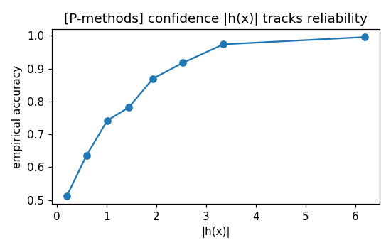
[P-methods] "Some ML methods inherently offer transparency": (a) a
            classification method quantifies the confidence of a
            classification via the distance |h(x)| of the feature
            vector from the decision boundary — predictions far from
            the boundary are empirically far more reliable than
            near-boundary ones, so disclosing this distance (as the
            entry's medical example requires) is informative; (b) a
            depth-2 decision tree is printable as human-readable
            if-then rules that exactly reproduce its predictions.
[P-read]    Art. 13 in the entry's Fig. 1: the learned hypothesis
            h(x) = 1 + 3.5(1 - exp(-0.35 x)) maps an applicant's
            income x' = 2.3 to a predicted credit score below the
            approval threshold 3.8, and the deployer can read off the
            prediction and its distance from the threshold.
[P-train]   Art. 11 in the entry's Fig. 1: the drawn hypothesis has a
            far smaller average loss on the training set of completed
            loans than a constant prediction, and the shaded income
            range lies entirely outside the range covered by the
            training set — the limitation the documentation must
            state.
[P-cf]      Art. 86 in the entry's Fig. 1: the counterfactual income
            x'' at which h reaches the approval threshold is
            ln(5)/0.35 = 4.5984..., matching the diamond drawn at 4.6;
            predictions at incomes above x'' exceed the threshold, so
            the stated change indeed flips the decision.

Outputs
-------
transparency.png : preview figure (checking only).

Data generated by pythondemos/transparency.py.
"""

import numpy as np
import matplotlib

matplotlib.use("Agg")
import matplotlib.pyplot as plt
from pathlib import Path

OUT_DIR = Path(__file__).parent

rng = np.random.default_rng(42)
report = []


def check(name, ok):
    report.append((name, bool(ok)))
    print(f"  [{'ok' if ok else 'FAIL'}] {name}")
"Some ML methods inherently offer transparency": (a) a classification method quantifies the confidence of a classification via the distance |h(x)| of the feature vector from the decision boundary — predictions far from the boundary are empirically far more reliable than near-boundary ones, so disclosing this distance (as the entry's medical example requires) is informative; (b) a depth-2 decision tree is printable as human-readable if-then rules that exactly reproduce its predictions.
print("[P-methods] (a) classification: confidence via the distance "
      "|h(x)| from the decision boundary")
m = 4000
X = rng.normal(size=(m, 2))
w_true = np.array([2.0, -1.5])
p = 1 / (1 + np.exp(-(X @ w_true)))
y = (rng.uniform(size=m) < p).astype(float)
w = np.zeros(2)
for _ in range(400):                               # train a linear hypothesis
    s = 1 / (1 + np.exp(-(X @ w)))
    w -= 0.5 * X.T @ (s - y) / m                   # decrease the average loss
h = X @ w                                          # h(x) = w^T x
pred = (h > 0).astype(float)
lo = np.abs(h) < np.quantile(np.abs(h), 0.3)       # low-confidence tercile
hi = np.abs(h) > np.quantile(np.abs(h), 0.7)       # high-confidence tercile
acc_lo, acc_hi = np.mean(pred[lo] == y[lo]), np.mean(pred[hi] == y[hi])
print(f"    accuracy at low / high |h(x)|: {acc_lo:.2f} / {acc_hi:.2f}")
check("distance from the decision boundary quantifies reliability: "
      "far-from-boundary predictions are far more accurate",
      acc_hi > acc_lo + 0.15)
check("disclosing the distance separates confident from uncertain "
      "predictions (medical-example requirement)",
      acc_hi > 0.9)

print("[P-methods] (b) decision tree: human-readable rules")
x1_split, x2_split = 0.0, 0.5
def tree_predict(X):
    out = np.empty(len(X))
    for i, (a, b) in enumerate(X):
        if a <= x1_split:
            out[i] = 0.0 if b <= x2_split else 1.0
        else:
            out[i] = 1.0 if b <= x2_split else 0.0
    return out
rules = [
    f"IF x1 <= {x1_split} AND x2 <= {x2_split} THEN predict 0",
    f"IF x1 <= {x1_split} AND x2 >  {x2_split} THEN predict 1",
    f"IF x1 >  {x1_split} AND x2 <= {x2_split} THEN predict 1",
    f"IF x1 >  {x1_split} AND x2 >  {x2_split} THEN predict 0",
]
for r in rules:
    print("      " + r)
def rules_predict(X):
    out = np.empty(len(X))
    for i, (a, b) in enumerate(X):
        if a <= x1_split and b <= x2_split: out[i] = 0.0
        elif a <= x1_split: out[i] = 1.0
        elif b <= x2_split: out[i] = 1.0
        else: out[i] = 0.0
    return out
Xt = rng.normal(size=(500, 2))
check("the printed if-then rules exactly reproduce the tree's "
      "predictions on every input",
      np.array_equal(tree_predict(Xt), rules_predict(Xt)))
check("the rule list is small enough to read (4 rules, depth 2)",
      len(rules) == 4)
[P-methods] (a) classification: confidence via the distance |h(x)| from the decision boundary
    accuracy at low / high |h(x)|: 0.60 / 0.97
  [ok] distance from the decision boundary quantifies reliability: far-from-boundary predictions are far more accurate
  [ok] disclosing the distance separates confident from uncertain predictions (medical-example requirement)
[P-methods] (b) decision tree: human-readable rules
      IF x1 <= 0.0 AND x2 <= 0.5 THEN predict 0
      IF x1 <= 0.0 AND x2 >  0.5 THEN predict 1
      IF x1 >  0.0 AND x2 <= 0.5 THEN predict 1
      IF x1 >  0.0 AND x2 >  0.5 THEN predict 0
  [ok] the printed if-then rules exactly reproduce the tree's predictions on every input
  [ok] the rule list is small enough to read (4 rules, depth 2)
Art. 13 in the entry's Fig. 1: the learned hypothesis h(x) = 1 + 3.5(1 - exp(-0.35 x)) maps an applicant's income x' = 2.3 to a predicted credit score below the approval threshold 3.8, and the deployer can read off the prediction and its distance from the threshold.
print("[P-read] Art. 13: read off the prediction and its distance "
      "from the approval threshold")
def h_credit(x):
    return 1 + 3.5 * (1 - np.exp(-0.35 * x))
tau = 3.8                                          # approval threshold
x_prime = 2.3                                      # applicant's income
score = h_credit(x_prime)
print(f"    h({x_prime}) = {score:.2f}, threshold {tau}, "
      f"distance {tau - score:.2f}")
check("the applicant's predicted score falls below the approval "
      "threshold", score < tau)
check("the distance from the threshold is readable from h alone",
      np.isclose(tau - score, tau - h_credit(x_prime)))
[P-read] Art. 13: read off the prediction and its distance from the approval threshold
    h(2.3) = 2.94, threshold 3.8, distance 0.86
  [ok] the applicant's predicted score falls below the approval threshold
  [ok] the distance from the threshold is readable from h alone
Art. 11 in the entry's Fig. 1: the drawn hypothesis has a far smaller average loss on the training set of completed loans than a constant prediction, and the shaded income range lies entirely outside the range covered by the training set — the limitation the documentation must state.
print("[P-train] Art. 11: the hypothesis fits the training set; the "
      "shaded incomes are not covered by it")
train = np.array([(0.7, 1.5), (1.2, 2.5), (1.8, 2.4), (2.3, 3.2),
                  (2.9, 3.0), (3.4, 3.7), (3.9, 3.4), (4.4, 4.0),
                  (4.9, 3.7), (5.4, 4.2), (5.9, 3.9)])
x_tr, y_tr = train[:, 0], train[:, 1]
loss_h = np.mean((y_tr - h_credit(x_tr)) ** 2)
loss_const = np.mean((y_tr - y_tr.mean()) ** 2)
print(f"    average loss: hypothesis {loss_h:.3f} vs constant "
      f"{loss_const:.3f}")
check("the drawn hypothesis has smaller average loss on the training "
      "set than a constant prediction", loss_h < 0.5 * loss_const)
shaded_lo, shaded_hi = 6.8, 9.5                    # shaded region of Fig. 1
check("the shaded income range lies outside the range covered by the "
      "training set (documented limitation)", shaded_lo > x_tr.max())
[P-train] Art. 11: the hypothesis fits the training set; the shaded incomes are not covered by it
    average loss: hypothesis 0.056 vs constant 0.611
  [ok] the drawn hypothesis has smaller average loss on the training set than a constant prediction
  [ok] the shaded income range lies outside the range covered by the training set (documented limitation)
Art. 86 in the entry's Fig. 1: the counterfactual income x'' at which h reaches the approval threshold is ln(5)/0.35 = 4.5984..., matching the diamond drawn at 4.6; predictions at incomes above x'' exceed the threshold, so the stated change indeed flips the decision.
print("[P-cf] Art. 86: the counterfactual income at which h reaches "
      "the threshold")
x_cf = np.log(5) / 0.35                            # h(x_cf) = tau exactly
print(f"    x'' = ln(5)/0.35 = {x_cf:.4f}")
check("h reaches the approval threshold at the counterfactual income",
      np.isclose(h_credit(x_cf), tau))
check("matches the diamond drawn at income 4.6 in Fig. 1",
      abs(x_cf - 4.6) < 0.01)
check("the change flips the decision: every income above x'' is "
      "predicted above the threshold",
      np.all(h_credit(np.linspace(x_cf + 1e-6, 9.5, 200)) > tau))

# ------------------------------------------------------------ preview
fig, ax = plt.subplots(1, 2, figsize=(9.6, 3.2))
bins = np.quantile(np.abs(h), np.linspace(0, 1, 9))
accs = [np.mean(pred[(np.abs(h) >= a) & (np.abs(h) < b)]
        == y[(np.abs(h) >= a) & (np.abs(h) < b)])
        for a, b in zip(bins[:-1], bins[1:])]
ax[0].plot(0.5 * (bins[:-1] + bins[1:]), accs, "o-")
ax[0].set_xlabel("distance |h(x)| from the decision boundary")
ax[0].set_ylabel("empirical accuracy")
ax[0].set_title("[P-methods] distance from the boundary tracks reliability")
xs = np.linspace(0, 9.5, 200)
ax[1].plot(xs, h_credit(xs), "k-", label="learned hypothesis h")
ax[1].axhline(tau, ls=":", c="k", label=f"approval threshold {tau}")
ax[1].plot(x_tr, y_tr, "o", c="C0", label="training set")
ax[1].plot([x_prime], [h_credit(x_prime)], "s", c="C1",
           label="applicant x'")
ax[1].plot([x_cf], [tau], "D", c="C2", label="counterfactual x''")
ax[1].axvspan(shaded_lo, shaded_hi, color="0.9",
              label="not covered by training set")
ax[1].set_xlabel("income (feature x)")
ax[1].set_ylabel("credit score (label y)")
ax[1].set_title("[P-read/-train/-cf] the credit-scoring example of Fig. 1")
ax[1].legend(frameon=False, fontsize=7)
fig.tight_layout()
fig.savefig(OUT_DIR / "transparency.png", dpi=110)
print(f"\n{sum(ok for _, ok in report)}/{len(report)} checks passed")
assert all(ok for _, ok in report)
[P-cf] Art. 86: the counterfactual income at which h reaches the threshold
    x'' = ln(5)/0.35 = 4.5984
  [ok] h reaches the approval threshold at the counterfactual income
  [ok] matches the diamond drawn at income 4.6 in Fig. 1
  [ok] the change flips the decision: every income above x'' is predicted above the threshold

11/11 checks passed
P-cf writes when the script runs