P-misuse writes when the script runsDictionary of Applied Machine Learning · test set
Numerical companion to the entry test set: it recomputes what the entry states and prints one line per check
The Krems weather narrative of the entry: today's maximum temperature is the feature, the next day's maximum temperature the label, and the data generation is a known linear rule plus Gaussian noise, so the risk of any hypothesis is computable and every claim of the entry can be checked against it. One block per paragraph of the entry (marked [P...]), in order. Self-contained (numpy/matplotlib only), fixed seeds.
Run it with python3 testset.py, from any directory — it writes its output files into the current directory. Requires NumPy and Matplotlib only, and uses fixed seeds, so the printed numbers reproduce exactly. Download testset.py · Notebook · Open in Colab
One cell per block of the script: the code, and what that code printed when it last ran here
"""
testset.py -- numerical companion to the entry 'test set'.

The Krems weather narrative of the entry: today's maximum temperature is
the feature, the next day's maximum temperature the label, and the data
generation is a known linear rule plus Gaussian noise, so the risk of
any hypothesis is computable and every claim of the entry can be checked
against it. One block per paragraph of the entry (marked [P...]), in
order. Self-contained (numpy/matplotlib only), fixed seeds.

Blocks
------
[P-tuning]  Training and validation data points tune the learned
            hypothesis: the average loss on the points used for
            training and model selection understates the loss on fresh
            data points.
[P-def]     The definition's estimator claims: for a hypothesis learned
            and selected without reference to the test set, the test
            error is an unbiased estimator of the risk (mean over many
            fresh test sets matches the analytic risk); the validation
            error of the selected hypothesis is optimistic (its mean
            lies below the winner's risk), while the test error is not.
[P-size]    The concentration bound on the test-set size: for a loss
            with values in [0,1], the deviation of the test error from
            the risk stays within sqrt(log(2/delta)/(2 m)) in at least
            a 1-delta fraction of repeated test draws, and the typical
            deviation shrinks like 1/sqrt(m); the entry's typical
            50/25/25 split of 200 data points is printed.
[P-misuse]  Evaluating many candidate hypotheses on the test set and
            keeping the best turns the test set into a validation set:
            the reported minimum test error lies below the winner's
            risk, while a fresh test set restores an honest estimate.

Outputs
-------
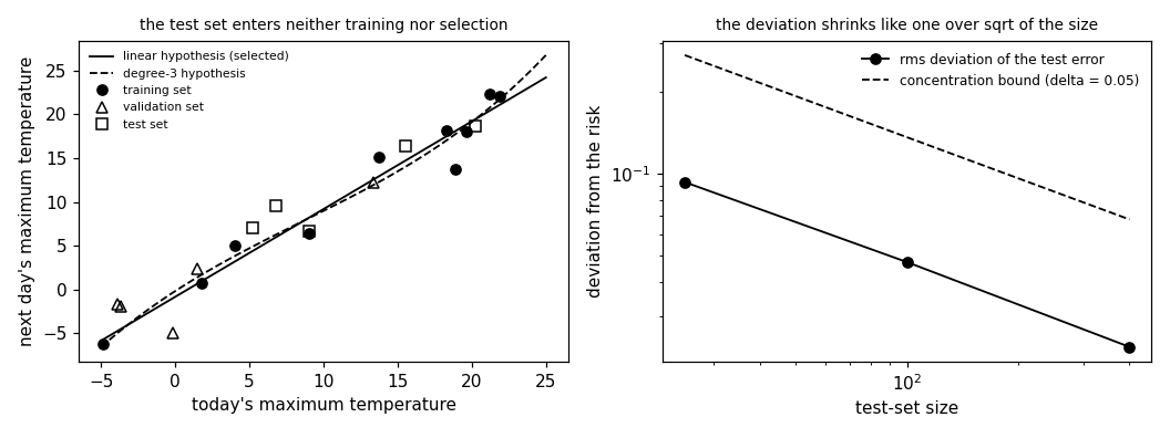
testset.png : preview figure (checking only).
"""

import numpy as np
import matplotlib

matplotlib.use("Agg")
import matplotlib.pyplot as plt

from math import erf
from pathlib import Path

OUT_DIR = Path(__file__).parent

report = []


def check(name, ok):
    report.append((name, bool(ok)))
    print(f"  [{'ok' if ok else 'FAIL'}] {name}")


# data generation: next day's maximum temperature from today's maximum
W0, W1, SIGMA = 1.5, 0.9, 2.5
X_LO, X_HI = -5.0, 25.0
XGRID = np.linspace(X_LO, X_HI, 20001)


def days(n, gen):
    x = gen.uniform(X_LO, X_HI, n)
    return x, W0 + W1 * x + gen.normal(0.0, SIGMA, n)


def sqerr(x, y, coeffs):
    return float(np.mean((y - np.polyval(coeffs, x)) ** 2))


def risk_sq(coeffs):
    """Risk under squared error: mean squared bias plus noise variance."""
    d = (W0 + W1 * XGRID) - np.polyval(coeffs, XGRID)
    return float(np.mean(d ** 2)) + SIGMA ** 2


PHI = np.vectorize(lambda t: 0.5 * (1.0 + erf(t / np.sqrt(2.0))))
BAND = 3.0


def banderr(x, y, coeffs):
    """0/1 loss: 1 if the prediction misses the label by more than BAND."""
    return float(np.mean(np.abs(y - np.polyval(coeffs, x)) > BAND))


def risk_band(coeffs):
    d = (W0 + W1 * XGRID) - np.polyval(coeffs, XGRID)
    inside = PHI((BAND - d) / SIGMA) - PHI((-BAND - d) / SIGMA)
    return float(np.mean(1.0 - inside))
Training and validation data points tune the learned hypothesis: the average loss on the points used for training and model selection understates the loss on fresh data points.
print("[P-tuning] the data points used for training and selection tune "
      "the learned hypothesis")

gen = np.random.default_rng(7)
x_tr, y_tr = days(10, gen)
x_va, y_va = days(5, gen)
c_lin = np.polyfit(x_tr, y_tr, 1)
c_pol = np.polyfit(x_tr, y_tr, 3)
c_sel = c_lin if sqerr(x_va, y_va, c_lin) <= sqerr(x_va, y_va, c_pol) \
    else c_pol
used = sqerr(np.r_[x_tr, x_va], np.r_[y_tr, y_va], c_sel)
print(f"    average loss on the used data points {used:.2f}, "
      f"risk {risk_sq(c_sel):.2f}")
check("the used data points make the hypothesis look better than fresh ones",
      used < risk_sq(c_sel))
[P-tuning] the data points used for training and selection tune the learned hypothesis
    average loss on the used data points 4.73, risk 8.79
  [ok] the used data points make the hypothesis look better than fresh ones
The definition's estimator claims: for a hypothesis learned and selected without reference to the test set, the test error is an unbiased estimator of the risk (mean over many fresh test sets matches the analytic risk); the validation error of the selected hypothesis is optimistic (its mean lies below the winner's risk), while the test error is not.
print("\n[P-def] the test error is an unbiased estimator of the risk; "
      "the validation error is not")

gen = np.random.default_rng(17)
testerrs = [sqerr(*days(25, gen), c_sel) for _ in range(3000)]
mean_test, r_sel = float(np.mean(testerrs)), risk_sq(c_sel)
se = float(np.std(testerrs)) / np.sqrt(3000.0)
print(f"    mean test error over 3000 fresh test sets {mean_test:.3f}, "
      f"risk {r_sel:.3f}")
check("mean test error matches the risk (within 3 standard errors)",
      abs(mean_test - r_sel) < 3 * se)

gen = np.random.default_rng(27)
gap_val, gap_test = [], []
for _ in range(400):
    xr, yr = days(20, gen)
    xv, yv = days(10, gen)
    cands = [np.polyfit(xr, yr, deg) for deg in range(5)]
    verrs = [sqerr(xv, yv, c) for c in cands]
    win = cands[int(np.argmin(verrs))]
    gap_val.append(min(verrs) - risk_sq(win))
    gap_test.append(sqerr(*days(25, gen), win) - risk_sq(win))
print(f"    winner's validation error minus risk, averaged: "
      f"{np.mean(gap_val):.2f}; test error minus risk: "
      f"{np.mean(gap_test):.2f}")
check("the validation error of the selected hypothesis is optimistic",
      np.mean(gap_val) < -0.5)
check("the test error of the selected hypothesis is not",
      abs(np.mean(gap_test)) < 0.2)
[P-def] the test error is an unbiased estimator of the risk; the validation error is not
    mean test error over 3000 fresh test sets 8.883, risk 8.788
  [ok] mean test error matches the risk (within 3 standard errors)
    winner's validation error minus risk, averaged: -1.02; test error minus risk: 0.06
  [ok] the validation error of the selected hypothesis is optimistic
  [ok] the test error of the selected hypothesis is not
The concentration bound on the test-set size: for a loss with values in [0,1], the deviation of the test error from the risk stays within sqrt(log(2/delta)/(2 m)) in at least a 1-delta fraction of repeated test draws, and the typical deviation shrinks like 1/sqrt(m); the entry's typical 50/25/25 split of 200 data points is printed.
print("\n[P-size] the concentration bound sizes the test set")

DELTA = 0.05
r_band = risk_band(c_sel)
rms = {}
gen = np.random.default_rng(37)
for m in (25, 100, 400):
    devs = np.array([banderr(*days(m, gen), c_sel) - r_band
                     for _ in range(3000)])
    rms[m] = float(np.sqrt(np.mean(devs ** 2)))
    if m == 100:
        bnd = np.sqrt(np.log(2.0 / DELTA) / (2.0 * m))
        cover = float(np.mean(np.abs(devs) <= bnd))
        print(f"    m = {m}: bound {bnd:.3f}, deviation within the bound "
              f"in {100 * cover:.1f}% of draws")
        check("the deviation stays within the bound in at least 95% of draws",
              cover >= 1.0 - DELTA)
print(f"    rms deviation: m=100 gives {rms[100]:.4f}, "
      f"m=400 gives {rms[400]:.4f}")
check("the typical deviation shrinks like one over sqrt of the size",
      abs(rms[100] / rms[400] - 2.0) < 0.5)
m_all = 200
print(f"    typical split of {m_all} data points: "
      f"{m_all // 2} training, {m_all // 4} validation, {m_all // 4} test")
[P-size] the concentration bound sizes the test set
    m = 100: bound 0.136, deviation within the bound in 99.8% of draws
  [ok] the deviation stays within the bound in at least 95% of draws
    rms deviation: m=100 gives 0.0473, m=400 gives 0.0232
  [ok] the typical deviation shrinks like one over sqrt of the size
    typical split of 200 data points: 100 training, 50 validation, 50 test
Evaluating many candidate hypotheses on the test set and keeping the best turns the test set into a validation set: the reported minimum test error lies below the winner's risk, while a fresh test set restores an honest estimate.
print("\n[P-misuse] keeping the best of many candidates turns the test "
      "set into a validation set")

gen = np.random.default_rng(47)
gap_reported, gap_fresh = [], []
for _ in range(300):
    cands = [np.array([W1 + gen.normal(0.0, 0.15),
                       W0 + gen.normal(0.0, 1.5)]) for _ in range(40)]
    xt, yt = days(20, gen)
    terrs = [sqerr(xt, yt, c) for c in cands]
    win = cands[int(np.argmin(terrs))]
    gap_reported.append(min(terrs) - risk_sq(win))
    gap_fresh.append(sqerr(*days(20, gen), win) - risk_sq(win))
print(f"    reported minimum test error minus the winner's risk, averaged: "
      f"{np.mean(gap_reported):.2f}; on a fresh test set: "
      f"{np.mean(gap_fresh):.2f}")
check("the reported minimum test error understates the winner's risk",
      np.mean(gap_reported) < -0.5)
check("a fresh test set restores an honest estimate",
      abs(np.mean(gap_fresh)) < 0.3)

# ------------------------------------------------------------------ preview
fig, axes = plt.subplots(1, 2, figsize=(9.6, 3.6))
ax = axes[0]
xs = np.linspace(X_LO, X_HI, 200)
ax.plot(xs, np.polyval(c_lin, xs), "-", color="black", lw=1.2,
        label="linear hypothesis (selected)")
ax.plot(xs, np.polyval(c_pol, xs), "--", color="black", lw=1.2,
        label="degree-3 hypothesis")
ax.plot(x_tr, y_tr, "o", ms=6, color="black", label="training set")
ax.plot(x_va, y_va, "^", ms=7, markerfacecolor="none",
        markeredgecolor="black", label="validation set")
x_te, y_te = days(5, np.random.default_rng(57))
ax.plot(x_te, y_te, "s", ms=6, markerfacecolor="none",
        markeredgecolor="black", label="test set")
ax.set_xlabel("today's maximum temperature")
ax.set_ylabel("next day's maximum temperature")
ax.set_title("the test set enters neither training nor selection",
             fontsize=9)
ax.legend(frameon=False, fontsize=7)

ax = axes[1]
ms = np.array(sorted(rms))
ax.loglog(ms, [rms[m] for m in ms], "o-", color="black", lw=1.2,
          label="rms deviation of the test error")
ax.loglog(ms, np.sqrt(np.log(2.0 / DELTA) / (2.0 * ms)), "--",
          color="black", lw=1.2, label="concentration bound (delta = 0.05)")
ax.set_xlabel("test-set size")
ax.set_ylabel("deviation from the risk")
ax.set_title("the deviation shrinks like one over sqrt of the size",
             fontsize=9)
ax.legend(frameon=False, fontsize=8)

fig.tight_layout()
fig.savefig(OUT_DIR / "testset.png", dpi=110)

n_ok = sum(ok for _, ok in report)
print(f"\n{n_ok}/{len(report)} checks pass")
print("wrote testset.png")
if n_ok != len(report):
    raise SystemExit(1)
[P-misuse] keeping the best of many candidates turns the test set into a validation set
    reported minimum test error minus the winner's risk, averaged: -1.08; on a fresh test set: -0.03
  [ok] the reported minimum test error understates the winner's risk
  [ok] a fresh test set restores an honest estimate

8/8 checks pass
wrote testset.png
P-misuse writes when the script runs